2.3: Standard Curve
- Page ID
- 38631
\( \newcommand{\vecs}[1]{\overset { \scriptstyle \rightharpoonup} {\mathbf{#1}} } \) \( \newcommand{\vecd}[1]{\overset{-\!-\!\rightharpoonup}{\vphantom{a}\smash {#1}}} \)\(\newcommand{\id}{\mathrm{id}}\) \( \newcommand{\Span}{\mathrm{span}}\) \( \newcommand{\kernel}{\mathrm{null}\,}\) \( \newcommand{\range}{\mathrm{range}\,}\) \( \newcommand{\RealPart}{\mathrm{Re}}\) \( \newcommand{\ImaginaryPart}{\mathrm{Im}}\) \( \newcommand{\Argument}{\mathrm{Arg}}\) \( \newcommand{\norm}[1]{\| #1 \|}\) \( \newcommand{\inner}[2]{\langle #1, #2 \rangle}\) \( \newcommand{\Span}{\mathrm{span}}\) \(\newcommand{\id}{\mathrm{id}}\) \( \newcommand{\Span}{\mathrm{span}}\) \( \newcommand{\kernel}{\mathrm{null}\,}\) \( \newcommand{\range}{\mathrm{range}\,}\) \( \newcommand{\RealPart}{\mathrm{Re}}\) \( \newcommand{\ImaginaryPart}{\mathrm{Im}}\) \( \newcommand{\Argument}{\mathrm{Arg}}\) \( \newcommand{\norm}[1]{\| #1 \|}\) \( \newcommand{\inner}[2]{\langle #1, #2 \rangle}\) \( \newcommand{\Span}{\mathrm{span}}\)\(\newcommand{\AA}{\unicode[.8,0]{x212B}}\)
RELATED READING: Pages 40, 87-89
OBJECTIVES
Upon completion of this exercise, appropriate discussion, and related readings, the student will be able to:
- Collect data appropriate for construction of a standard curve.
- Use this data to construct a standard curve.
- Use a standard curve to determine the values for unknown solutions.
GLOSSARY
Semi-logarithmic graph: a graph in which one axis is a linear scale while the other axis is a logarithmic (log, to base 10) scale. The log scale may be 1, 2, or more cycles (factors of 10).
Stock solution: a primary solution of a compound or buffer, usually prepared in a concentrated form with pure solid or liquid compound. This solution is used to prepare more dilute, “working” solutions.
MATERIALS
- 16x 100 mm test tubes
- Stock KMnO4
- Pipets
- Distilled Water
- Spectrophotometer
- Unknown solutions
- Graph paper
PROCEDURES
- Label 16 x 100 mm test tubes one through five.
- Using a 5 mL serological or Mohr pipet, pipet stock solution into tubes one through four in the amounts shown below.
- Using another 5 mL serological or Mohr pipet, deliver distilled water into tubes 2, 3, 4, and 5 in the quantities shown.
DILUTION TABLE
| Tube | Stock Solution | Distilled Water | Final Concentration |
|---|---|---|---|
| 1 | 5.0 mL | 50 mg/L | |
| 2 | 4.0 mL | 1.0 mL | 40 mg/L |
| 3 | 3.0 mL | 2.0 mL | 30 mg/L |
| 4 | 2.0 mL | 3.0 mL | 20 mg/L |
| 5 | 1.0 mL | 4.0 mL | 10 mg/L |
- Mix each solution well.
- Adjust the spectrophotometer to 540 nm and zero it with a distilled water blank.
- Pour each solution Into a cuvette and read the absorbance and transmittance of each.
- Record your results on the data sheet.
- Read the absorbance and transmittance of the assigned unknown solutions and record them on the data sheet.
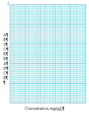
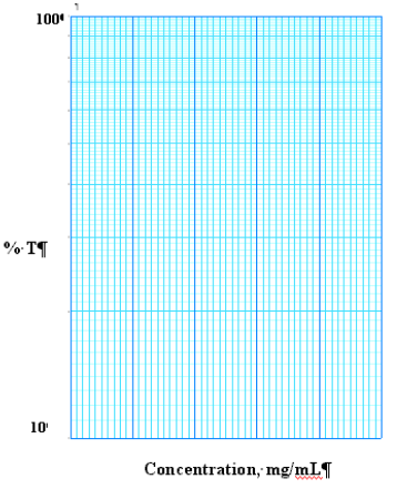
- Using the values for your stock dilutions, plot absorbance vs. concentration on the linear graph paper and transmittance vs. concentration on semi-logarithmic graph paper; both graph papers can be found at the end of this exercise.
- Using the graphs you have constructed, determine the concentration of each of the unknowns.
| DATA SHEET, EXERCISE #3 |
NAME: ___________ DATE: ___________ |
STANDARDS
| CONCENTRATION | ||
|---|---|---|
| (mg/L) | Absorbance | Transmittance |
| 5.0 | ||
| 4.0 | ||
| 3.0 | ||
| 2.0 | ||
| 1.0 | ||
UNKNOWNS
| Absorbance | Transmittance | Concentration | |
|---|---|---|---|
| Unknown # | |||
| Unknown # | |||
| Unknown # |
Discussion Questions
- Why were different types of graph paper used?
- Is the absorbance of KMnO4 linear over the concentration range used for this lab?
- Why was a wavelength of 540 nm used?
- Compare the calculation method of determining concentration used in exercise 1 with the standard curve method you have just performed. What are the advantages and disadvantages of each? Which will yield a more accurate answer? Why?


