
3.6: Computed Tomography (CT)
- Page ID
- 14799

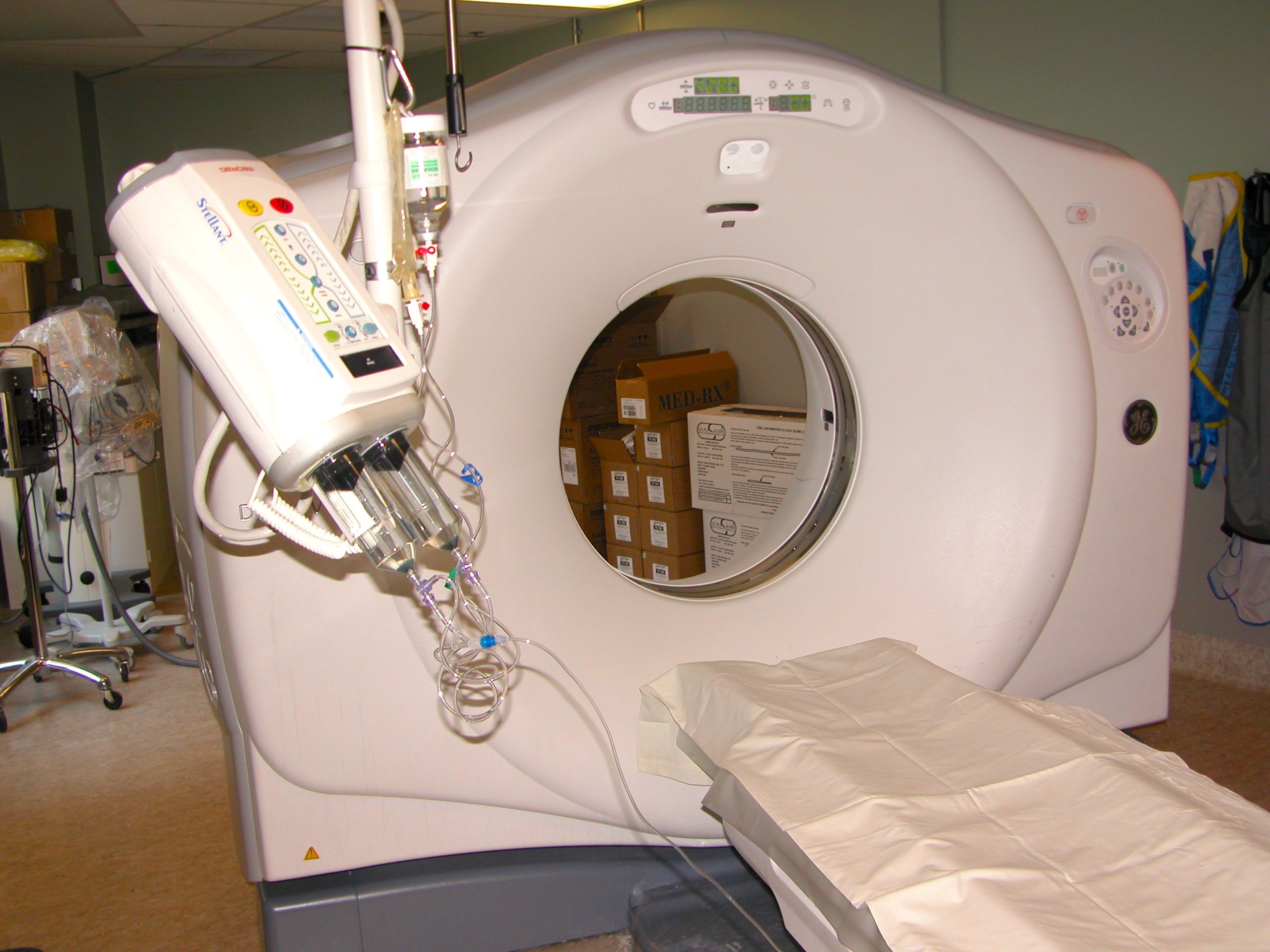
CT relies upon x-rays to facilitate image creation. The x-ray tube is situated in a ring assembly that is able to spin around the horizontal table that the patient lies on. The x-ray tube generates x-rays only when programmed and activated by a CT Technologist. The detectors for the x-rays that pass through the patient are located in the ring structure and rotate in unison with the source of the x-rays. The whole assembly that holds the x-ray tube and x-ray detectors is in the large doughnut shaped part of the unit called, the gantry. At the same time that the tube and detectors spin the horizontal table top that the patient lies on moves slowly through the gantry ring. This rotating x-ray source, associated with the rotating detectors, and the horizontally moving table top is called a helical CT scanner. This imaging device is presented in Figure 3.21.
The patient does not need to be moved, or re-positioned, to obtain CT images in different anatomic planes. The patient lies on the CT table in anatomic position and remains in that position throughout the study. The standard orientation of image acquisition for CT is in the axial plane, hence the old name for this machine of CAT (computed axial tomography) scanner. Often the axial images obtained during the initial x-ray exposure will be digitally reformatted into other anatomic planes i.e. sagittal and coronal. These reformatted images are the result of a computer algorithm reformatting the original digital image data and, as such, these supplemental anatomic planes of imaging do not require additional x-ray exposure.
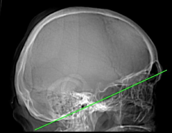
The CT gantry can be tipped cranially and caudally to deviate from the axial plane by 30 degrees in either direction and this can be used to correct for patient anatomic variability to maintain the axial plane, if necessary. It also allows for unique imaging along an angled plane that can be used when requested by the referring physician or the radiologist. A widely used example of imaging in an angled plane is found for CT Head examinations. It is not conventional to acquire these images in the axial plane but to image the brain on the canthomeatal (lateral orbit canthus to the aural meatus) line and therefore, the CT gantry must be tilted to ensure that all CT Head images are acquired in this plane. Originally, this plane was chosen as it maximizes information about the intra-cranial contents while minimizing the exposure of the orbits (lens) to radiation. The orbito-meatal line has become the internationally recognized plane for acquiring CT head images. This line is depicted in Figure 3.22.
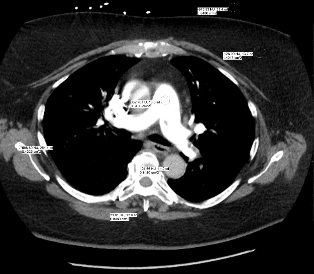
The physics of CT image creation are complex and require complex computer processing to create images that are visible for clinical use. As the x-ray tube and the x-ray detectors revolve around the patient thousands of mathematical calculations are performed to determine how much of the incident x-ray beam was absorbed by a volume of tissue. This volume of tissue is called a voxel. The calculated absorption of the x-rays by a voxel is converted into a pixel density that is displayed on a gray scale from -1,000 (air) to +1,000 (metal). This scale is called the Hounsfield unit (HU) scale after one of the principle inventors of CT, Sir Godfrey Hounsfield. The calculated density of this voxel is then allocated to a pixel on a grid of the 512 x 512 pixels that forms each individual CT image.
Therefore, if the volume of tissue contained air, or gas, the pixel density allocated would be close to -1,000 HU, while if the volume of tissue analyzed contained metal (bullet fragment, etc.) the pixel would be assigned a density close to the +1,000 HU. The assignment of pixel density to voxels spans the entire possible range of pixels from -1,000 – +1,000 HU, resulting in 2,000 shades of grey. An image with the HU measurements of specific anatomic regions is provided in Figure 3.23.
CT density: a region on a CT image is described as being more, or less, dense than another region. The liver is more dense than the renal cortex. This variation in pixel density can be quantified by measuring all the pixels in a region and creating an average pixel density i.e. region of interest of an area of liver can be measured, with a standard deviation, 50 HU +/- 5 HU, etc. The HU density of some common structures is provided in Table 3.2.
| – 1000 | Air |
|---|---|
| – 600 | Lung |
| – 120 to – 90 | Fat |
| 0 | Water |
| – 5 to 15 | Bile |
| 10 to 15 | CSF |
| 20 to 40 | Soft Tissue |
| 20 to 30 | White Matter |
| 37 to 45 | Grey Matter |
| 40 | Old Blood |
| 80 to 100 | Acute Blood |
| 700 | Medullary Bone |
| 800 | Cortical Bone |
| 1000 | Metal |
The viewer of the CT can decide how to adjust the level and window of the displayed CT images to accentuate tissues of a defined pixel density. The level and window are at the discretion of the viewing radiologist and can be set to their preferences. There are a variety of established level and window settings, i.e. abdomen, bone, brain, etc. These help to provide some level of uniformity for comparison of multiple CT examinations. Level and window setting for six common tissues are as follows:
| Anatomy | Level | Window |
|---|---|---|
| Abdomen | 40 | 400 |
| Bone | 300 | 2000 |
| Brain | 35 | 80 |
| Liver | 50 | 200 |
| Lung | -700 | 1500 |
| PE | 50 | 351 |
CT images demonstrating the appearance of these six different level and window settings are provided in Figure 3.24.
 Abdomen Level/Width |
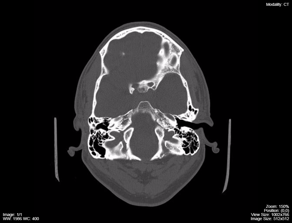 Bone Level/Width |
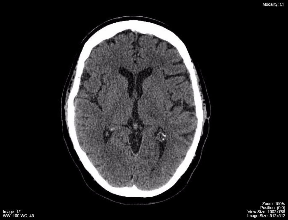 Brain Level/Width |
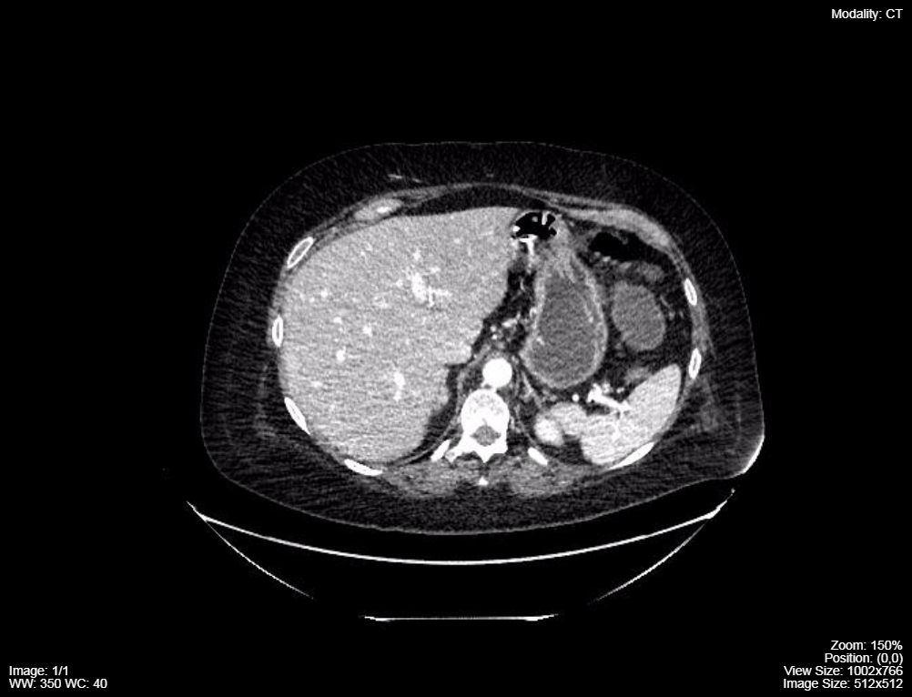 Liver Level/Width |
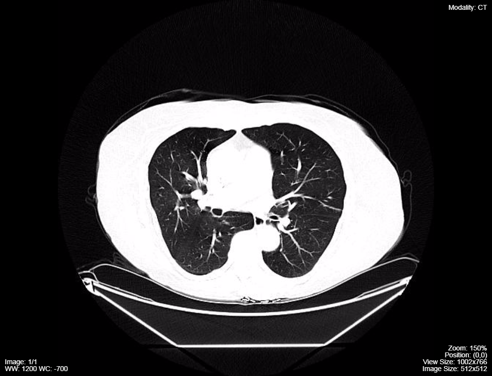 Lung Level/Width |
 PE Level/Width |
Figure 3.24 CT images with different level and window settings
ODIN Link for Figure 3.24: mistr.usask.ca/odin/?caseID=20170706145901557
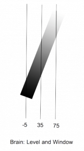
Level and Window are unique physical properties of CT images that allow the user to adjust the centre and the width of the gray scale that is portrayed on the images. This is an adjustment that is applied to the raw CT data and does not require repeated patient imaging to obtain the different levels and windows. The level is the centre of the gray scale, set to the HU of the tissue of most interest i.e. the centre (level) of the gray scale for brain window is 35 HU. The window is the width of the gray scale that surrounds the level setting, thus defining the range of HU for white and black seen on the image. For the brain images the width of the HU scale is 80 HU. A illustration depicting this for brain and bone level and window setting are provided in Figure 3.25.
Brain
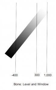
Bone
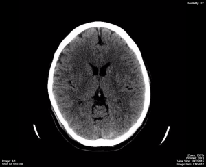
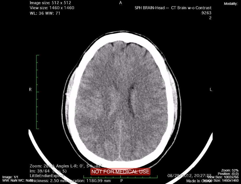
Once the window range is set, any structures with a pixel density greater than the defined window will appear white and everything with a pixel density less than the defined window will appear black. The ability to adjust the range of greys that are displayed on the image, makes it possible for the interpreter to analyze and compare structures of interest. It is important to remember that when viewing images on a particular level and window setting the anatomy of structures that fall outside the gray scale you are viewing will not be optimally analyzed. This is particularly evident when you assess the difference in appearance of the head images provided demonstrating the brain and the bone level and window settings. Brain tissue is well visualized on the brain level and window while there is no useful information about the bone of the skull and vice versa when the bone level and window is viewed, see Figure 3.26.
Brain
Bone
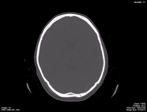
ODIN Link for Figure 3.26: mistr.usask.ca/odin/?caseID=20170714073330478
It is important to realize the effect of level and window and review the image data set provided to you at all the appropriate level and window settings. For example, in the thorax one should view the images on lung, mediastinal, and bone level and window settings to perform a full assessment of the patient’s anatomy.
The standard viewing format for the CT image display is to look at the images like a loaf of sliced bread with the observer standing at the foot end of the table while the patient is in anatomic position. Therefore, the patient’s right sided anatomy is on the left side when looking at the display monitor. The image is marked with a R (right), L (left), A (anterior), and P (posterior) indicators to orient the viewer. See Figure 3.27.
CT imaging administers a high radiation exposure to the patient compared to other imaging modalities. The best way to limit patient radiation exposure is to not image excessive anatomy i.e. plan the CT scan to image as little anatomy as possible. Newer CT scanners have the ability to adjust the x-ray dose administered based upon the changes in volume and thickness of the patient anatomy. Also, newer scanners can use software algorithms to reformat images obtained with very low dose radiation and achieve diagnostic quality.
There are two major technical features of the CT data set that helps to minimize overall patient radiation exposure:
a) The images are obtained as such thin slices, so closely aligned to each other, that the digital data can be reformatted with software in the coronal and sagittal planes with resulting very high image quality. Therefore, the patient only requires one dose of radiation to achieve visualization of their anatomy in the axial, coronal, and sagittal planes, this minimizing overall radiation exposure. (See Figure 3.28)
Axial
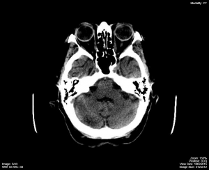
Sagittal
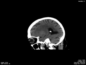
Coronal

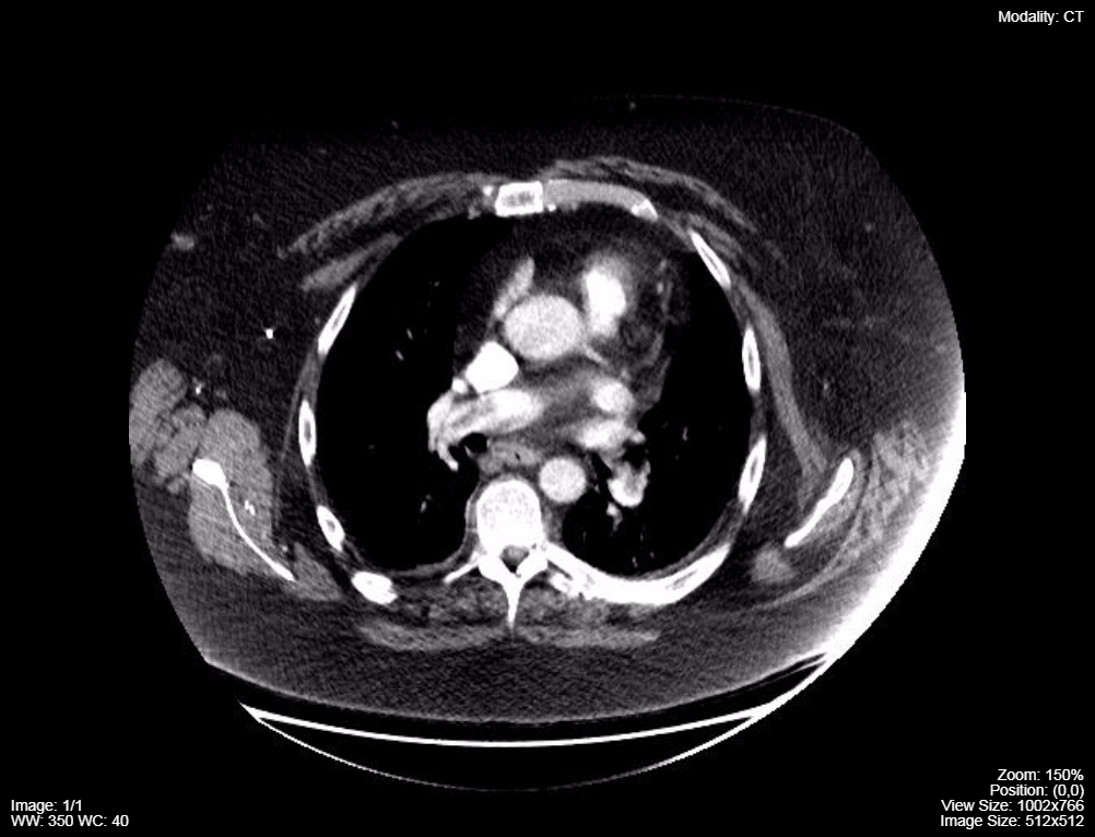
ODIN Link for Figures 3.28A – C: mistr.usask.ca/odin/?caseID=20160216170931060 b) The level/window settings can be adjusted for each individual image, regardless of the displayed plane of imaging, to best demonstrate a wide variety of anatomy, i.e. bone, lung, abdomen, mediastinum, etc. This again provides maximum utility of the images acquired from a single radiation dose. (See figure 3.29) Lung

Mediastinum
Computed Tomographic Angiography
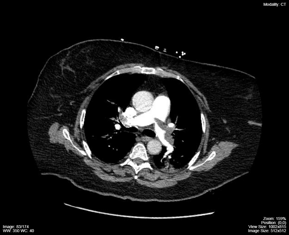
CT has also become highly adapted to imaging arterial and venous anatomy and in some instances has replaced catheter based angiography as the gold standard examination, e.g. pulmonary angiography has been supplanted by CT PE (pulmonary embolism) studies. This is due to the ability of the newer, multi-detector, helical, CT scanners to rapidly cover a large area of patient anatomy due to the size of the detectors. Hence, contrast enhanced CT images can be obtained during a narrow window of time when a particular vascular structure is maximally enhanced with intravenous contrast agent. The image acquisition can be timed to maximally enhance arteries or veins. Figure 3.30 demonstrates optimal timing of the CT images for enhancement of the pulmonary arteries.
Computed Tomography:
- Takes images in an axial format, and re-formats them into sagittal and coronal images
- Uses the Hounsfield Unit scale (HU) to assign densities to tissues
- Hounsfield Units range from -1000 (air) to +1000 (metal) with 0 assigned to water
Image Appearance:
- 6 standard level/window settings for assessing various structures, however any user specified level/window setting can be used
- Abdomen, Bone, Brain, Liver, Lungs, Pulmonary Embolism (PE)
- Level refers to the Hounsfield Unit the image is centered on
- Window refers to the range of Hounsfield Units displayed on either side of the Level
- When viewing CT images, the patient’s right is on the left side of the display monitor
Radiation Exposure:
- Reduced by setting the CT x-ray dose to as low as feasible to minimize the total radiation exposure
- The CT Technologist can minimize the total volume of tissue irradiated by setting the margins of the imaged anatomy to as small a region as feasible
- One set of images can be reformatted in different anatomic planes and adjusted (level/window) to optimally view the anatomy without additional x-ray exposure
Computed Tomography Angiography (CTA):
- Useful for the assessment arterial imaging such as, the pulmonary arteries for Pulmonary Embolism (PE), intra-cranial arteries for aneurysms, and cervical arteries for narrowing, occlusion, or dissection, etc.
- Uses contrast that is injected into the venous system
Attributions
Fig 3.21 Helical CT Scanner by Dr. Brent Burbridge MD, FRCPC, University Medical Imaging Consultants, College of Medicine, University of Saskatchewan is used under a CC-BY-NC-SA 4.0 license.
Fig 3.22 The plane of imaging related to the cantho-meatal line by Dr. Brent Burbridge MD, FRCPC, University Medical Imaging Consultants, College of Medicine, University of Saskatchewan is used under a CC-BY-NC-SA 4.0 license.
Fig 3.23 Images of CT with HU measurements by Dr. Brent Burbridge MD, FRCPC, University Medical Imaging Consultants, College of Medicine, University of Saskatchewan is used under a CC-BY-NC-SA 4.0 license.
Fig 3.24 CT Images with different level and window settings by Dr. Brent Burbridge MD, FRCPC, University Medical Imaging Consultants, College of Medicine, University of Saskatchewan is used under a CC-BY-NC-SA 4.0 license.
Fig 3.25A Brain Level and Window by Dr. Brent Burbridge MD, FRCPC, University Medical Imaging Consultants, College of Medicine, University of Saskatchewan is used under a CC-BY-NC-SA 4.0 license.
Fig 3.25B Bone Level and Window by Dr. Brent Burbridge MD, FRCPC, University Medical Imaging Consultants, College of Medicine, University of Saskatchewan is used under a CC-BY-NC-SA 4.0 license.
Fig 3.26A Head CT visible on brain level and window. Bone not well seen by Dr. Brent Burbridge MD, FRCPC, University Medical Imaging Consultants, College of Medicine, University of Saskatchewan is used under a CC-BY-NC-SA 4.0 license.
Fig 3.26B Head CT on bone level and window. Brain not well seen by Dr. Brent Burbridge MD, FRCPC, University Medical Imaging Consultants, College of Medicine, University of Saskatchewan is used under a CC-BY-NC-SA 4.0 license.
Fig 3.27 Standard viewing orientation for an axial CT image by Dr. Brent Burbridge MD, FRCPC, University Medical Imaging Consultants, College of Medicine, University of Saskatchewan is used under a CC-BY-NC-SA 4.0 license.
Fig 3.28A CT image displayed in axial orientation from one radiation exposure event by Dr. Brent Burbridge MD, FRCPC, University Medical Imaging Consultants, College of Medicine, University of Saskatchewan is used under a CC-BY-NC-SA 4.0 license.
Fig 3.28B CT image displayed in sagittal orientation from one radiation exposure event by Dr. Brent Burbridge MD, FRCPC, University Medical Imaging Consultants, College of Medicine, University of Saskatchewan is used under a CC-BY-NC-SA 4.0 license.
Fig 3.28C CT image displayed in coronal orientation from one radiation exposure event by Dr. Brent Burbridge MD, FRCPC, University Medical Imaging Consultants, College of Medicine, University of Saskatchewan is used under a CC-BY-NC-SA 4.0 license.
Fig 3.29A CT of the chest on lung level/window by Dr. Brent Burbridge MD, FRCPC, University Medical Imaging Consultants, College of Medicine, University of Saskatchewan is used under a CC-BY-NC-SA 4.0 license.
Fig 3.29B CT of the chest on mediastinal level/window by Dr. Brent Burbridge MD, FRCPC, University Medical Imaging Consultants, College of Medicine, University of Saskatchewan is used under a CC-BY-NC-SA 4.0 license.
Fig 3.30 CT PE image maximizing the injected contrast in the pulmonary arteries by Dr. Brent Burbridge MD, FRCPC, University Medical Imaging Consultants, College of Medicine, University of Saskatchewan is used under a CC-BY-NC-SA 4.0 license.