5.6: Interventions allocated to groups

The methods described in Sections 3 to 5 all assume that individuals are to be the units of allocation. In other words, the trial groups will be constructed effectively by making a complete list of the individuals available for the trial and randomly selecting which individuals are to be allocated to each trial group. As explained in Chapter 4, Section 4, however, many field trials are not organized in this way. Instead, groups of individuals are allocated to the interventions under study. These groups are often called clustersand may correspond to communities, for example, villages, hamlets, or defined sectors of an urban area; institutions such as schools or workplaces; or patients attending a particular health facility.

Trials in which communities or other types of cluster are randomly allocated to the different arms of the trial are known as cluster randomized trials, and sample size calculations for such trials are presented in Section 6.1. Stepped wedge trials are a modified form of cluster randomized trial and are discussed in Section 6.2.

6.1 Cluster randomized trials

If clusters are randomly allocated to the different trial arms, the cluster should also be used as the unit of analysis, even though assessments of outcome are made on individu- als within clusters (see Chapter 21, Section 8). For example, suppose the mosquito-net trial is to be conducted as follows. A number of villages (say 20) are to be randomly divided into two equal-sized groups. In the ten villages in the first group, the entire population of each village will be given mosquito-nets, while the second group of ten villages will serve as controls. The analysis of the impact of mosquito-nets on the in- cidence of clinical malaria would be made by calculating the (age-adjusted) incidence rate in each village and comparing the ten rates for the intervention villages with the ten rates for the control villages. This would be achieved by treating the (age-adjusted) rate as the quantitative outcome measured for each village and comparing these, using the unpaired t-test or the non-parametric rank sum test (see Chapter 21, Section 8). If analysing proportions, rather than incidence rates, the principle is the same—the (age- adjusted) proportion would be treated as the quantitative outcome for each cluster.

When allocation is by cluster, the trial size formulae have to be adjusted to allow for intrinsic variation between communities. Suppose first that incidence rates in the two groups are to be compared. The required number of clusters c is given by:

\[
c=1+\left(z_{1}+z_{2}\right)^{2}\left[\left(r_{1}+r_{2}\right) / y+k^{2}\left(r_{1}^{2}+r_{2}^{2}\right)\right] /\left(r_{1}-r_{2}\right)^{2}
\]

In this formula, y is the person-years of observation in each cluster, while r1 and r2are the average rates in the intervention and control clusters, respectively. The intrinsic variation between clusters is measured by k, the coefficient of variation of the (true) incidence rates among the clusters in each group, and is defined as the standard devia- tion of the rates divided by the average rate. The value of k is assumed similar in the intervention and control groups, so that the relative variability remains the same fol- lowing intervention.

If proportions are to be compared, the required number of clusters is given by:

\[
c=1+\left(z_{1}+z_{2}\right)^{2}\left[2 p(1-p) / n+k^{2}\left(p_{1}^{2}+p_{2}^{2}\right)\right] /\left(p_{1}-p_{2}\right)^{2}
\]

In this formula, n is the trial size in each community; p1 and p2 are the average proportions in the intervention and control groups, respectively; p is the average of p1and p2 , and k is the coefficient of variation of the (true) proportions among the clusters in each group.

An estimate of k will sometimes be available from previous data on the same clusters or from a pilot study. If no data are available, it may be necessary to make an arbitrary, but plausible, assumption about the value of k. For example, k = 0.25 implies that the true rates in each group vary roughly between ri ±2kri , i.e. between 0.5r and 1.5r. In general, k is unlikely to exceed 0.5.

Example: Suppose the mosquito-net trial is to be conducted by allocating the inter- vention at the village level. The incidence rate of clinical malaria among children before intervention is 10 per 1000 child-weeks of observation, and the trial is to be designed to give 90% power if the intervention reduces the incidence rate by 50%. There are about 50 eligible children per village, and it is intended to continue follow-up for 1 year, so that y is approximately 2500 child-weeks. No information is available on between- village variation in incidence rates. Taking , the number of villages required per group is given by the following, so that roughly seven villages would be needed in each group:

\[
c=1+(1.96+1.28)^{2}\left[(0.01+0.005) / 2500+0.25^{2}\left(0.01^{2}+0.005^{2}\right)\right] /(0.01-0.005)^{2}=6.8
\]

Note that this would give a total of 17 500 child-weeks of observation in each group, compared with 6300 child-weeks if individual children were randomized to receive mosquito-nets. Figure 5.2 shows the number of villages required in each group, de- pending on the child-weeks of observation per village and the value of k.

The effect of group allocation on the total trial size needed will depend on the degree to which individuals within a cluster are more likely to be similar to each other than individuals in a different cluster for the outcome measure in the trial. If there is no het- erogeneity between clusters in the outcome of interest, in the sense that the variation between the cluster-specific rates or means is no more than would be expected to occur by chance, due to sampling variations, the total trial size will be approximately the same as if the interventions were allocated to individuals. For most outcomes, however, there will be real differences between clusters, and, in these circumstances, the required trial size will be greater than with individual allocation. The ratio of the required trial sizes with cluster and individual allocation is sometimes called the design effect. Unfortu- nately, no single value for the design effect can be assumed, as its value depends on the variability of the outcome of interest between clusters and on the sizes of the clusters, and so it is recommended that the required sample size is estimated explicitly.

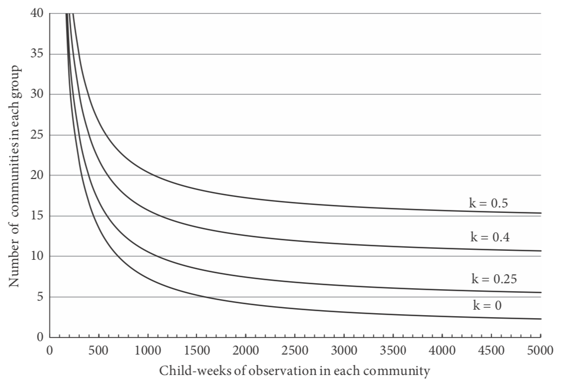
Figure 5.2 Number of communities required in each group in a trial of the effect of mosquito-nets against clinical malaria.

Note that, even if the calculations suggest that less than four clusters are required in each group, it is preferable to have at least four in each group. With so few units of ob- servation, the use of non-parametric procedures, such as the rank sum test, is generally preferred for the analysis, and a sample size of at least four in each group is needed to have any chance of obtaining a significant result when this test is used.

It may be possible to reduce the required number of communities by adopting a matched design. For example, this can be done by using the baseline study to arrange the clusters into pairs, in which the rates of the outcome of interest are similar, and randomly selecting one member of each pair to receive the intervention. However, it is difficult to quantify the effect of this approach on the number of clusters required. To do this, information is required on the variability of the treatment effect between com- munities and on the extent to which the baseline data are predictive of the rates that would be observed during the follow-up period in the absence of intervention, and this information is rarely available. With a paired design, at least six clusters are required in each group in order to be able to obtain a significant difference using a non-parametric statistical test.

Further information on sample size calculations for cluster randomized trials is given in Hayes and Bennett (1999) and Hayes and Moulton (2009).

According to the number of child-weeks of observation in each community and the extent of variation in rates of clinical malaria between communities (k is the coefficient of variation of the incidence rates; see text). The average incidence rate of clinical malaria in the absence of the intervention is assumed to be ten per 10 000 weeks of observation, and the trial is required to have 90% power to detect a 50% reduction in the incidence of malaria at the p < 0.05 level of statistical significance.

6.2 Stepped wedge trials

The stepped wedge design was introduced in Chapter 4, Section 4.3 and is a modi- fication of the cluster randomized trial, in which all clusters commence the trial in the control group. The intervention is then introduced gradually into the clusters in random order, until, at the end of the trial, all the clusters are in the intervention group.

A consequence of the stepped wedge design is that, at most time points during the trial, there will be unequal numbers of clusters in the intervention and control groups. This means that, when secular trends are accounted for by comparing intervention to control groups at each step, a stepped wedge trial can have lower power and precision than a standard cluster randomized trial of the same size, in which the numbers of in- tervention and control clusters are equal throughout. When there is zero intra-cluster correlation, the trial will need up to 50% more clusters. To adjust for this, the number of clusters has to be multiplied by a correction factor which depends on the number of ‘steps’ in the stepped wedge design. If there are five steps, the correction factor is 1.3, rising to approximately 1.4 for numbers of steps between 10 and 20. When intra-cluster correlation is large enough, the gain in efficiency that can be made by taking advantage of the pre–post information on each cluster can overtake this factor, making a stepped wedge trial more efficient than a parallel trial. To be conservative, however, it may be best to inflate the number of clusters.

Example: In the mosquito-net trial discussed earlier, the sample size calculation showed that we needed seven clusters in each arm or a total of 14 clusters. If we now propose to carry out this trial using a stepped wedge trial, a conservative correction would be to multiply this number by 1.4, giving 20 clusters. For example, this might be implemented with ten steps over a 5-year period, providing nets to two randomly chosen clusters each half year.