4.3: The eXtended Contrastive Attractor Learning (XCAL) Model

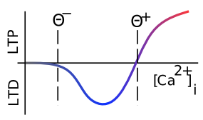
The learning function we adopt for the models in the rest of this text is called the eXtended Contrastive Attractor Learning (XCAL) rule. (The basis for this naming will become clear later). This learning function was derived through a convergence of bottom-up (motivated by detailed biological considerations) and top-down (motivated by computational desiderata) approaches. In the bottom-up derivation, we extracted an empirical learning function (called the XCAL dWt function) from a highly biologically detailed computational model of the known synaptic plasticity mechanisms, by Urakubo, Honda, Froemke, & Kuroda (2008) (see Detailed Biology of Learning for more details). Their model builds in detailed chemical rate parameters and diffusion constants, etc, based on empirical measurements, for all of the major biological processes involved in synaptic plasticity. We capture much of the incredible complexity of the Urakubo, Honda, Froemke, & Kuroda (2008) model (and by extension, hopefully, the complexity of the actual synaptic plasticity mechanisms in the brain) using a simple piecewise-linear function, shown below, that emerges from it. This XCAL dWt function closely resembles the function shown in Figure 4.2, plotting the dependence of synaptic plasticity on Ca++ levels. It also closely resembles the Bienenstock, Cooper, & Munro (1982) (BCM) learning function.

The top-down approach leverages the key idea behind the BCM learning function, which is the use of a floating threshold for determining the amount of activity needed to elicit LTP vs LTD (see Figure 4.2). Specifically, the threshold is not fixed at a particular value, but instead adjusts as a function of average activity levels of the postsynaptic neuron in question over a long time frame, resulting in a homeostatic dynamic. Neurons that have been relatively inactive can more easily increase their synaptic weights at lower activity levels, and can thus "get back in the game". Conversely, neurons that have been relatively overactive are more likely to decrease their synaptic weights, and "stop hogging everything".

As we'll see below, this function contributes to useful self-organizing learning, where different neurons come to extract distinct aspects of statistical structure in a given environment. But purely self-organizing mechanisms are strongly limited in what they can learn -- they are driven by statistical generalities (e.g., animals tend to have four legs), and are incapable of adapting more pragmatically to the functional demands that the organism faces. For example, some objects are more important to recognize than others (e.g., friends and foes are important, random plants or pieces of trash or debris, not so much).

To achieve these more pragmatic goals, we need error-driven learning, where learning is focused specifically on correcting errors, not just categorizing statistical patterns. Fortunately, we can use the same floating threshold mechanism to achieve error-driven learning within the same overall mathematical framework, by adapting the threshold on a faster time scale. In this case, weights are increased if activity states are greater than their very recent levels, and conversely, weights decrease if the activity levels go down relative to prior states. Thus, we can think of the recent activity levels (the threshold) as reflecting expectations which are subsequently compared to actual outcomes, with the difference (or "error") driving learning. Because both forms of learning (self-organizing and error-driven) are quite useful, and use the exact same mathematical framework, we integrate them both into a single set of equations with two thresholds reflecting integrated activity levels across different time scales (recent and long-term average).

Next, we describe the XCAL dWt function (dWt = change in weight), before describing how it captures both forms of learning, followed by their integration into a single unified framework (including the promised explanation for its name!).

The XCAL dWt Function

Figure \(4.4\): The XCAL dWt function, showing direction and magnitude of synaptic weight changes (dWt) as a function of the short-term average activity of the sending neuron (\(x\)) times the receiving neuron (\(y\)). This quantity is a simple mathematical approximation to the level of postsynaptic Ca++, reflecting the dependence of the NMDA channel on both sending and receiving neural activity. This function was extracted directly from the detailed biophysical Urakubo, Honda, Froemke, & Kuroda (2008) model, by fitting a piecewise linear function to the synaptic weight change behavior that emerges from it as a function of a wide range of sending and receiving spiking patterns.

The XCAL dWt function extracted from the Urakubo, Honda, Froemke, & Kuroda (2008) model is shown in Figure 4.4. First, the main input into this function is the total synaptic activity reflecting the firing rate and duration of activity of the sending and receiving neurons. In mathematical terms for a rate-code model with sending activity rate x and receiving activity rate y, this would just be the "Hebbian" product we described above:

• \(\Delta w=f_{x c a l}\left(x y, \theta_{p}\right)\)

where \(f_{x c a l}\) is the piecewise linear function shown in Figure 4.4. The weight change also depends on an additional dynamic threshold parameter \(\theta_{p}\), which determines the point at which it crosses over from negative to positive weight changes -- i.e., the point at which weight changes reverse sign. For completeness, here is the mathematical expression of this function, but you only need to understand its shape as shown in the figure:

• \(f_{x c a l}\left(x y, \theta_{p}\right)=\left\{\begin{array}{ll}{\left(x y-\theta_{p}\right)} & {\text { if } x y>\theta_{p} \theta_{d}} \\ {-x y\left(1-\theta_{d}\right) / \theta_{d}} & {\text { otherwise }}\end{array}\right.\)

where \(\theta_{d}=.1\)is a constant that determines the point where the function reverses direction (i.e., back toward zero within the weight decrease regime) -- this reversal point occurs at \(\theta_{p} \theta_{d}\), so that it adapts according to the dynamic \(\theta_{p}\) value.

As noted in the previous section, the dependence of the NMDA channel on activity of both sending and receiving neurons can be summarized with this simple Hebbian product, and the level of intracellular Ca++ is likely to reflect this value. Thus, the XCAL dWt function makes very good sense in these terms: it reflects the qualitative nature of weight changes as a function of Ca++ that has been established from empirical studies and postulated by other theoretical models for a long time. The Urakubo model simulates detailed effects of pre/postsynaptic spike timing on Ca++ levels and associated LTP/LTD, but what emerges from these effects at the level of firing rates is this much simpler fundamental function.

As a learning function, this basic XCAL dWt function has some advantages over a plain Hebbian function, while sharing its basic nature due to the "pre * post" term at its core. For example, because of the shape of the dWt function, weights will go down as well as up, whereas the Hebbian function only causes weights to increase. But it still has the problem that weights will increase without bound (as long as activity levels are often greater than the threshold). We'll see in the next section that some other top-down computationally-motivated modifications can result in a more powerful form of learning while maintaining this basic form.

Self-Organizing Learning: Long Time Scales and the BCM Model

Figure \(4.5\): The shape of the BCM learning function. Note the similarity in qualitative shape to both the XCAL dWt function and synaptic plasticity as function of Ca++.

The major computational motivation comes from a line of learning functions that began with Bienenstock, Cooper, & Munro (1982), with these initials giving rise to the name of the function: BCM. (Interestingly Leon Cooper, a Nobel Laurate in Physics, was also "central" in the BCS theory of superconductivity). The BCM function is a modified form of Hebbian learning, which includes an interesting homeostatic mechanism that keeps individual neurons from firing too much or too little over time:

• \(\Delta w=x y(y-\theta)\)

where again \(x\) = sending activity, \(y\) = receiving activity, and \(\theta\) is a floating threshold reflecting a long time average of the receiving neuron's activity:

• \(\theta=\left\langle y^{2}\right\rangle\)

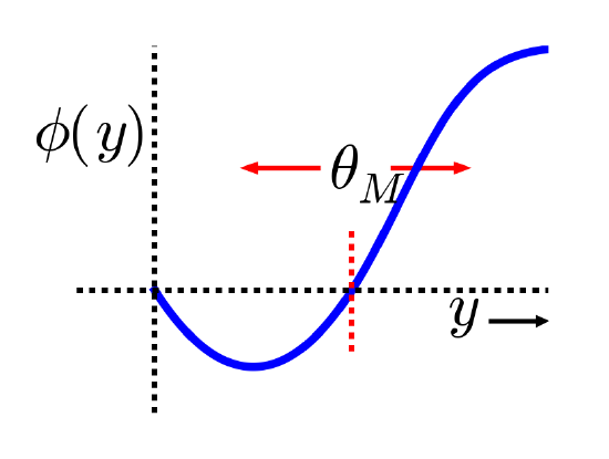
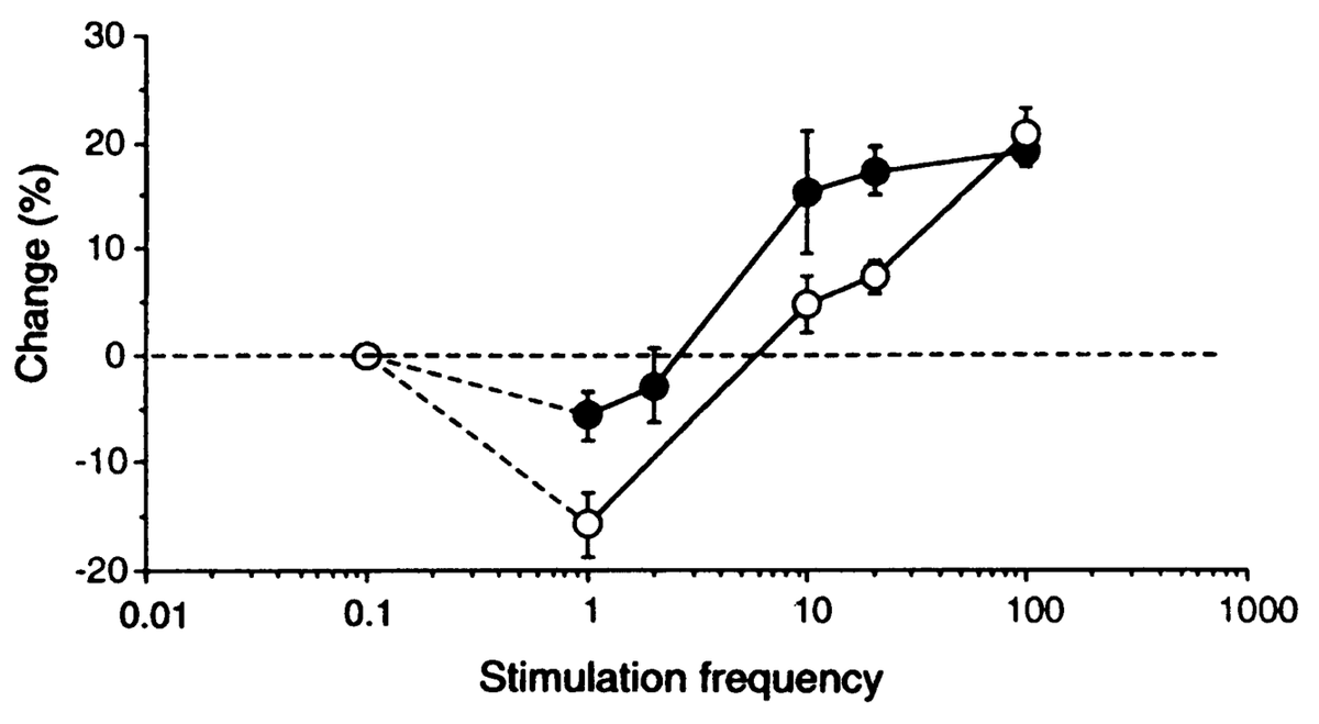
where \(\langle \rangle\) indicates the expected value or average, in this case of the square of the receiving neuron's activation. Figure 4.5 shows what this function looks like overall -- a shape that should be becoming rather familiar. Indeed, the fact that the BCM learning function anticipated the qualitative nature of synaptic plasticity as a function of Ca++ (Figure 4.2) is an amazing instance of theoretical prescience. Furthermore, BCM researchers have shown that it does a good job of accounting for various behavioral learning phenomena, providing a better fit than a comparable Hebbian learning mechanism (Figure 4.6, (Cooper, Intrator, Blais, & Shouval, 2004) ).

Figure \(4.6\): Synaptic plasticity data from dark reared (filled circles) and normally-reared (open circles) rats, showing that dark reared rats appear to have a lower threshold for LTP, consistent with the BCM floating threshold. Neurons in these animals are presumably much less active overall, and thus their threshold moves down, making them more likely to exhibit LTP relative to LTD. Reproduced from Kirkwood, Rioult, & Bear (1996).

BCM has typically been applied in simple feedforward networks in which, given an input pattern, there is only one activation value for each neuron. But how should weights be updated in a more realistic bidirectionally connected system with attractor dynamics in which activity states continuously evolve through time? We confront this issue in the XCAL version of the BCM equations:

• \(\Delta w=f_{x c a l}\left(x y,\langle y\rangle_{l}\right)=f_{x c a l}\left(x y, y_{l}\right)\)

where \(x y\) is understood to be the short-term average synaptic activity (on a time scale of a few hundred milliseconds -- the time scale of Ca++ accumulation that drives synaptic plasticity), which could be more formally expressed as: \(\langle x y\rangle_{s}\), and \(y_{l}=\langle y\rangle_{l}\) is the long-term average activity of the postsynaptic neuron (i.e., essentially the same as in BCM, but without the squaring), which plays the role of the \(\theta_{p}\) floating threshold value in the XCAL function.

After considerable experimentation, we have found the following way of computing the \(y_{l}\) floating threshold to provide the best ability to control the threshold and achieve the best overall learning dynamics:

• \(\begin{array}{l}{\text { if } y>.2 \text { then } y_{l}=y_{l}+\frac{1}{\tau_{l}}\left(\max -y_{l}\right)} \\ {\text { else } y_{l}=y_{l}+\frac{1}{\tau}\left(\min -y_{l}\right)}\end{array}\)

This produces a well-controlled exponential approach to either the max or min extremes depending on whether the receiving unit activity exceeds the basic activity threshold of .2. The time constant for integration \(\tau_{l}\) is 10 by default -- integrating over around 10 trials. See XCAL_Details sub-topic for more discussion.

Figure \(4.7\): How the floating threshold as a function of long-term average receiver neural activity \(\langle y\rangle_{l}\) drives homeostatic behavior. Neurons that have low average activity are much more likely to increase their weights because the threshold is low, while those that have high average activity are much more likely to decrease their weights because the threshold is high.

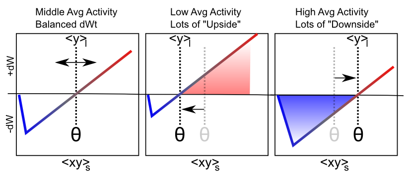
Figure 4.7 shows the main qualitative behavior of this learning mechanism: when the long term average activity of the receiver is low, the threshold moves down, and thus it is more likely that the short term synaptic activity value will fall into the positive weight change territory. This will tend to increase synaptic weights overall, and thus make the neuron more likely to get active in the future, achieving the homeostatic objective. Conversely, when the long term average activity of the receiver is high, the threshold is also high, and thus the short term synaptic activity is more likely to drive weight decreases than increases. This will take these over-active neurons down a notch or two, so they don't end up dominating the activity of the network.

Self-organizing Learning Dynamics

This ability to spread the neural activity around in a more equitable fashion turns out to be critical for self-organizing learning, because it enables neurons to more efficiently and effectively cover the space of things to represent. To see why, here are the critical elements of the self-organizing learning dynamic (see subsequent simulation exploration to really get a feel for how this all works in practice):

• Inhibitory competition -- only the most strongly driven neurons get over the inhibitory threshold, and can get active. These are the ones whose current synaptic weights best fit ("detect") the current input pattern.
• Rich get richer positive feedback loop -- due to the nature of the learning function, only those neurons that actually get active are capable of learning (when receiver activity y = 0, then xy = 0 too, and the XCAL dWt function is 0 at 0). Thus, the neurons that already detect the current input the best are the ones that get to further strengthen their ability to detect these inputs. This is the essential insight that Hebb had with why the Hebbian learning function should strengthen an "engram".
• homeostasis to balance the positive feedback loop -- if left unchecked, the rich-get-richer dynamic ends up with a few units dominating everything, and as a result, all the inputs get categorized into one useless, overly-broad category ("everything"). The homeostatic mechanism in BCM helps fight against this by raising the floating threshold for highly active neurons, causing their weights to decrease for all but their most preferred input patterns, and thus restoring a balance. Similarly, under-active neurons experience net weight increases that get them participating and competing more effectively, and hence they come to represent distinct features.

The net result is the development of a set of neural detectors that relatively evenly cover the space of different inputs patterns, with systematic categories that encompass the statistical regularities. For example, cats like milk, and dogs like bones, and we can learn this just by observing the reliable co-occurrence of cats with milk and dogs with bones. This kind of reliable co-occurrence is what we mean by "statistical regularity". See Hebbian Learning for a very simple illustration of why Hebbian-style learning mechanisms capture patterns of co-occurrence. It is really just a variant on the basic maxim that "things that fire together, wire together".

The Learning Rate

There is an important factor missing from the above equations, which is the learning rate -- we typically use the Greek epsilon \(\epsilon\) to represent this parameter, which simply multiplies the rate with which the weights change:

• \(\Delta w=\epsilon f_{x c a l}\left(x y, y_{l}\right)\)

Thus, a bigger epsilon means larger weight changes, and thus quicker learning, and vice-versa for a smaller value. A typical starting value for the learning rate is .04, and we often have it decrease over time (which is true of the brain as well -- younger brains are much more plastic than older ones) -- this typically results in the fastest overall learning and best final performance.

Many researchers (and drug companies) have the potentially dangerous belief that a faster learning rate is better, and various drugs have been developed that effectively increase the learning rate, causing rats to learn some kind of standard task faster than normal, for example. However, we will see in the Learning and Memory Chapter that actually a slow learning rate has some very important advantages. Specifically, a slower learning rate enables the system to incorporate more statistics into learning -- the learning rate determines the effective time window over which experiences are averaged together, and a slower learning rate gives a longer time window, which enables more information to be integrated. Thus, learning can be much smarter with a slower learning rate. But the tradeoff of course is that the results of this smarter learning take that much longer to impact actual behavior. Many have argued that humans are distinctive in our extremely protracted period of developmental learning, so we can learn a lot before we need to start earning a paycheck. This allows us to have a pretty slow learning rate, without too many negative consequences.

Exploration of Self-Organizing Learning

The best way to see this dynamic is via the computational exploration. Open the Self Organizing simulation and follow the directions from there.

Error-Driven Learning: Short Time Scale Floating Threshold

Although self-organizing learning is very useful, we'll see that it is significantly limited in the kinds of things that it can learn. It is great for extracting generalities, but not so great when it comes to learning specific, complicated patterns. To learn these more challenging types of problems, we need error-driven learning. For a more top-down (computationally motivated) discussion of how to achieve error-driven learning, and relationship to the more biologically motivated mechanisms we consider here, see the Backpropagation subsection (which some may prefer to read first). Intuitively, error-driven learning is much more powerful because it drives learning based on differences, not raw signals. Differences (errors) tell you much more precisely what you need to do to fix a problem. Raw signals (overall patterns of neural activity) are not nearly as informative -- it is easy to become overwhelmed by the forest and lose sight of the trees. We'll see more specific examples later, after first figuring out how we can get error-driven learning to work in the first place.

Figure \(4.8\): How the floating threshold as a function of medium-term average synaptic activity \(\langle x y\rangle_{m}\) can produce error-driven learning. This medium time frame reflects the development of a pattern of neural activity that encodes an expectation about what will happen next. The most recent short term synaptic activity (which drives learning) represents the actual outcome of what did happen next. Because of the (nearly) linear nature of the dWt function, it effectively computes the difference between outcome and expectation. Qualitatively, if the outcome produces greater activation of a population of neurons than did expectation, corresponding weights go up, while neurons that decreased their activity states as a result of the outcome will have their weights go down. This is illustrated above in the case of low vs. high expectations.

Figure 4.8 shows how the same floating threshold behavior from the BCM-like self-organizing aspect of XCAL learning can be adapted to perform error-driven learning, in the form of differences between an outcome vs. an expectation. Specifically, we speed up the time scale for computing the floating threshold (and also have it reflect synaptic activity, not just receiver activity):

• \(\Theta_{p}=\langle x y\rangle_{m}\)
• \(\Delta w=f_{x c a l}\left(\langle x y\rangle_{s},\langle x y\rangle_{m}\right)=f_{x c a l}\left(x_{s} y_{s}, x_{m} y_{m}\right)\)

where \(\langle x y\rangle_{m}\) is this new medium-time scale average synaptic activity, which we think of as reflecting an emerging expectation about the current situation, which develops over approximately 75 msec of neural activity. The most recent, short-term (last 25 msec) neural activity (\(\langle x y\rangle_{s}\)) reflects the actual outcome, and it is the same calcium-based signal that drives learning in the Hebbian case.

In the simulator, the period of time during which this expectation is represented by the network, before it gets to see the outcome, is referred to as the minus phase (based on the Boltzmann machine terminology; (Ackley, Hinton, & Sejnowski, 1985)). The subsequent period in which the outcome is observed (and the activations evolve to reflect the influence of that outcome) is referred to as the plus phase. It is the difference between this expectation and outcome that represents the error signal in error-driven learning (hence the terms minus and plus -- the minus phase activations are subtracted from those in the plus phase to drive weight changes).

Although this expectation-outcome comparison is the fundamental requirement for error-driven learning, a weight change based on this difference by itself begs the question of how the neurons would ever 'know' which phase they are in. We have explored many possible answers to this question, and the most recent involves an internally-generated alpha-frequency (10 Hz, 100 msec periods) cycle of expectation followed by outcome, supported by neocortical circuitry in the deep layers and the thalamus (O'Reilly, Wyatte, & Rohrlich, 2014; Kachergis, Wyatte, O'Reilly, Kleijn, & Hommel, 2014). A later revision of this textbook will describe this in more detail. For now, the main implications of this framework are to organize the timing of processing and learning as follows:

• A Trial lasts 100 msec (10 Hz, alpha frequency), and comprises one sequence of expectation -- outcome learning, organized into 4 quarters.

• Biologically, the deep neocortical layers (layers 5, 6) and the thalamus have a natural oscillatory rhythm at the alpha frequency (Buffalo, Fries, Landman, Buschman, & Desimone, 2011; Lorincz, Kekesi, Juhasz, Crunelli, & Hughes, 2009; Franceschetti et al., 1995; Luczak, Bartho, & Harris, 2013). Specific dynamics in these layers organize the cycle of expectation vs. outcome within the alpha cycle.

• A Quarter lasts 25 msec (40 Hz, gamma frequency) -- the first 3 quarters (75 msec) form the expectation / minus phase, and the final quarter are the outcome / plus phase.

• Biologically, the superficial neocortical layers (layers 2, 3) have a gamma frequency oscillation (Buffalo, Fries, Landman, Buschman, & Desimone, 2011), supporting the quarter-level organization.

• A Cycle represents 1 msec of processing, where each neuron updates its membrane potential according to the equations covered in the Neuron chapter.

The XCAL learning mechanism coordinates with this timing by comparing the most recent synaptic activity (predominantly driven by plus phase / outcome states) to that integrated over the medium-time scale, which effectively includes both minus and plus phases. Because the XCAL learning function is (mostly) linear, the association of the floating threshold with this synaptic activity over the medium time frame (including expectation states), to which the short-term outcome is compared, directly computes their difference:

• \(\Delta w \approx x_{s} y_{s}-x_{m} y_{m}\)

Intuitively, we can understand how this error-driven learning rule works by thinking about different specific cases. The easiest case is when the expectation is equivalent to the outcome (i.e., a correct expectation) -- the two terms above will be the same, and thus their subtraction is zero, and the weights remain the same. So once you obtain perfection, you stop learning. What if your expectation was higher than your outcome? The difference will be a negative number, and the weights will thus decrease, so that you will lower your expectations next time around. Intuitively, this makes perfect sense -- if you have an expectation that all movies by M. Night Shyamalan are going to be as cool as The Sixth Sense, you might end up having to reduce your weights to better align with actual outcomes. Conversely, if the expectation is lower than the outcome, the weight change will be positive, and thus increase the expectation. You might have thought this class was going to be deadly boring, but maybe you were amused by the above mention of M. Night Shyamalan, and now you'll have to increase your weights just a bit. It should hopefully be intuitively clear that this form of learning will work to minimize the differences between expectations and outcomes over time. Note that while the example given here was cast in terms of deviations from expectations having value (ie things turned out better or worse than expected, as we cover in more detail in the Motor control and Reinforcement Learning chapter, the same principle applies when outcomes deviate from other sorts of expectations.

Because of its explicitly temporal nature, there are a few other interesting ways of thinking about what this learning rule does, in addition to the explicit timing defined above. To reiterate, the rule says that the outcome comes immediately after a preceding expectation -- this is a direct consequence of making it learn toward the short-term (most immediate) average synaptic activity, compared to a slightly longer medium-term average that includes the time just before the immediate present.

Figure \(4.9\): Illustration of Contrastive Attractor Learning (CAL) principle, which is core idea behind XCAL error-driven learning mechanism. The network learns on the contrast between the early phase of settling (the minus phase, or medium time frame activation average \(\langle x y\rangle_{m}\)) versus the late phase of settling (the plus phase or short time frame activation average \(\langle x y\rangle_{s}\)). The late phase has integrated more of the overall constraints in the network and thus represents a "better" overall interpretation or representation of the current situation than the early phase, so it makes sense for the late phase to serve as the "training signal" relative to the earlier phase.

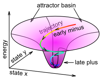
We can think of this learning in terms of the attractor dynamics discussed in the Networks Chapter. Specifically, the name Contrastive Attractor Learning (CAL) reflects the idea that the network is settling into an attractor state, and it is the contrast between the final attractor state that the network settles into (i.e., the "outcome" in this case), versus the network's activation trajectory as it approaches the attractor, that drives learning (Figure 4.9). The short-time scale average reflects the final attractor state (the 'target'), and the medium time-scale average reflects the entire trajectory during settling. When the pattern of activity associated with the expectation is far from the actual outcome, the difference between these two attractor states will be large, and learning will drive weight changes so that in future encounters, the expectation will more closely reflect the outcome (assuming the environment is reliable). The X part of XCAL simply reflects the fact that the same objective is achieved without having to explicitly compare two attractors at discrete points in time, but instead by using a time-averaged activity state eXtended across the entire settling trajectory as the baseline comparison, which is more biologically realistic because such variables are readily accessible by local neuronal activity.

Mathematically, this CAL learning rule represents a simpler version of the oscillating learning function developed by Norman and colleagues -- see Oscillating Learning Function for more details.

There are also more general reasons for later information (short time scale average) to train earlier information (medium time scale average). Typically, the longer one waits, the better quality the information is -- at the start of a sentence, you might have some idea about what is coming next, but as it unfolds, the meaning becomes clearer and clearer. This later information can serve to train up the earlier expectations, so that you can more efficiently understand things next time around. Overall, these alternative ways of thinking about XCAL learning represent more self-organizing forms of learning without requiring an explicit outcome training signal, while using the more rapid contrast (short vs. medium time) for the error-driven learning mechanism.

Before continuing, you might be wondering about the biological basis of this error-driven form of the floating threshold. Unlike the BCM-style floating threshold, which has solid empirical data consistent with it, the idea that the threshold changes on this quicker time scale to reflect the medium time-scale average synaptic activity has not yet been tested empirically. Thus, it stands as an important prediction of this computational model. Because it is so easily computed, and results in such a powerful form of learning, it seems plausible that the brain would take advantage of just such a mechanism, but we'll have to see how it stands up to empirical testing. One initial suggestion of such a dynamic comes from this paper: Lim et al. (2015), which showed a BCM-like learning dynamic with rapid changes in the threshold depending on recent activity. Also, there is substantial evidence that transient changes in neuromodulation that occur during salient, unexpected events, are important for modifying synaptic plasticity -- and may functionally contribute to this type of error-driven learning mechanism. Also, we discuss a little bit later another larger concern about the nature and origin of the expectation vs. outcome distinction, which is central to this form of error-driven learning.

Advantages of Error-Driven Learning

As noted above, error-driven learning is much more computationally powerful than self-organizing learning. For example, all computational models that perform well at the difficult challenge of learning to recognize objects based on their visual appearance (see Perception Chapter) utilize a form of error-driven learning. Many also use self-organizing learning, but this tends to play more of a supporting role, whereas the models would be entirely non-functional without error-driven learning. Error-driven learning ensures that the model makes the kinds of categorical discriminations that are relevant, while avoiding those that are irrelevant. For example, whether a side view of a car is facing left or right is not relevant for determining that this is a car. But the presence of wheels is very important for discriminating a car from a fish. A purely self-organizing model has no way of knowing that these differences, which may be quite statistically reliable and strong signals in the input, differ in their utility for the categories that people care about.

Mathematically, the history of error-driven learning functions provides a fascinating window into the sociology of science, and how seemingly simple ideas can take a while to develop. In the Backpropagation subsection, we trace this history through the derivation of error-driven learning rules, from the delta rule (developed by Widrow and Hoff in 1960) to the very widely used backpropagation learning rule (Rumelhart et al., 1986). At the start of that subsection, we show how the XCAL form of error-driven learning (specifically the CAL version of it) can be derived directly from backpropagation, thus providing a mathematically satisfying account as to why it is capable of solving so many difficult problems.

The key idea behind the backpropagation learning function is that error signals arising in an output layer can propagate backward down to earlier hidden layers to drive learning in these earlier layers so that it will solve the overall problem facing the network (i.e., it will ensure that the network can produce the correct expectations or answers on the output layer). This is essential for enabling the system as a whole to solve difficult problems -- as we discussed in the Networks Chapter, a lot of intelligence arises from multiple layers of cascading steps of categorization -- to get all of these intervening steps to focus on the relevant categories, error signals need to propagate across these layers and shape learning in all of them.

Figure \(4.10\): Intuition for how bidirectional connections enable the backpropagation of learning signals from other parts of the network -- when there is a difference between an expectation and an outcome in any part of the network, neurons in other parts of the network "feel" that difference via the bidirectional connection. All neurons experience an impact on their own activation of both the expectation and the outcome, and thus when they learn on the difference between these two points in time (later training earlier), they are learning about their own impact on the outcome - expectation error, and weight changes based on this difference will end up minimizing the overall error in the network as a whole. Neurons closer to the source of the error learn the most, with error decreasing with distance from this source.

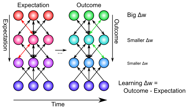
Biologically, the bidirectional connectivity in our models enables these error signals to propagate in this manner (Figure 4.10). Thus, changes in any given location in the network radiate backward (and every which way the connections go) to affect activation states in all other layers, via bidirectional connectivity, and this then influences the learning in these other layers. In other words, XCAL uses bidirectional activation dynamics to communicate error signals throughout the network, whereas backpropagation uses a biologically implausible procedure that propagates error signals backward across synaptic connections, in the opposite direction of the way that activation typically flows. Furthermore, the XCAL network experiences a sequence of activation states, going from an expectation to experiencing a subsequent outcome, and learns on the difference between these two states. In contrast, backpropagation computes a single error delta value that is effectively the difference between the outcome and the expectation, and then sends this single value backwards across the connections. See the Backpropagation subsection for how these two different things can be mathematically equivalent. Also, it is a good idea to look at the discussion of the credit assignment process in this subsection, to obtain a fuller understanding of how error-driven learning works.

Exploration of Error-Driven Learning

The Pattern Associator simulation provides a nice demonstration of the limitations of self-organizing Hebbian-style learning, and how error-driven learning overcomes these limitations, in the context of a simple two-layer pattern associator that learns basic input/output mappings. Follow the directions in that simulation link to run the exploration.

You should have seen that one of the input/output mapping tasks was impossible for even error-driven learning to solve, in the two-layer network. The next exploration, Error Driven Hidden shows that the addition of a hidden layer, combined with the powerful error-driven learning mechanism, enables even this "impossible" problem to now be solved. This demonstrates the computational power of the Backpropagation algorithm.

Combined Self-Organizing and Error-Driven Learning

Although scientists have a tendency to want to choose sides strongly and declare that either self-organizing learning or error-driven learning is the best way to go, there are actually many advantages to combining both forms of learning together. Each form of learning has complementary strengths and weaknesses:

• Self-organizing is more robust, because it only depends on local statistics of firing, whereas error-driven learning implicitly depends on error signals coming from potentially distant areas. Self-organizing can achieve something useful even when the error signals are remote or not yet very coherent.
• But self-organizing learning is also very myopic -- it does not coordinate with learning in other layers, and thus tends to be "greedy". In contrast, error-driven learning achieves this coordination, and can learn to solve problems that require collective action of multiple units across multiple layers.

One analogy that may prove useful is that error-driven learning is like left-wing politics -- it requires all the different layers and units to be working together to achieve common goals, whereas self-organizing learning is like right-wing politics, emphasizing local, greedy actions that somehow also benefit society as a whole, without explicitly coordinating with others. The tradeoffs of these political approaches are similar to those of the respective forms of learning. Socialist approaches can leave individual people feeling not very motivated, as they are just a little cog in a huge faceless machine. Similarly, neurons that depend strictly on error-driven learning can end up not learning very much, as they only need to make a very small and somewhat "anonymous" contribution to solving the overall problem. Once the error signals have been eliminated (i.e., expectations match outcomes), learning stops. We will see that networks that rely on pure error-driven learning often have very random-looking weights, reflecting this minimum of effort expended toward solving the overall problem. On the other side, more strongly right-wing capitalist approaches can end up with excessive positive feedback loops (rich get ever richer), and are typically not good at dealing with longer-term, larger-scale problems that require coordination and planning. Similarly, purely self-organizing models tend to end up with more uneven distributions of "representational wealth" and almost never end up solving challenging problems, preferring instead to just greedily encode whatever interesting statistics come their way. Interestingly, our models suggest that a balance of both approaches -- a centrist approach -- seems to work best! Perhaps this lesson can be generalized back to the political arena.

Colorful analogies aside, the actual mechanics of combining both forms of learning within the XCAL framework amounts to merging the two different definitions of the floating threshold value. Biologically, we think that there is a combined weighted average of the two thresholds, using a "lambda" parameter \(\lambda\) to weight the long-term receiver average (self-organizing) relative to the medium-term synaptic co-product:

• \(\theta_{p}=\lambda y_{l}+(1-\lambda) x_{m} y_{m}\)

However, computationally, it is clearer and simpler to just combine separate XCAL functions, each with their own weighting function -- due to the linearity of the function, this is mathematically equivalent:

• \(\Delta w=\lambda_{f} f_{x c a l}\left(x_{s} y_{s}, y_{l}\right)+\lambda_{m} f_{x c a l}\left(x_{s} y_{s}, x_{m} y_{m}\right)\)

It is reasonable that these lambda parameters may differ according to brain area (i.e., some brain systems learn more about statistical regularities, whereas others are more focused on minimizing error), and even that it may be dynamically regulated (i.e. transient changes in neuromodulators like dopamine and acetylcholine can influence the degree to which error signals are emphasized).

There are small but reliable computational advantages to automating this balancing of self-organizing vs. error-driven learning (i.e., a dynamically-computed \(\lambda_{l}\) value, while keeping \(\lambda_{m}=1\)), based on two factors: the magnitude of the y_l receiving-unit running average activation, and the average magnitude of the error signals present in a layer (see Leabra Details).

Weight Bounding and Contrast Enhancement

The one last issue we need to address computationally is the problem of synaptic weights growing without bound. In LTP experiments, it is clear that there is a maximum synaptic weight value -- you cannot continue to get LTP on the same synapse by driving it again and again. The weight value saturates. There is a natural bound on the lower end, for LTD, of zero. Mathematically, the simplest way to achieve this kind of weight bounding is through an exponential approach function, where weight changes become exponentially smaller as the bounds are approached. This function is most directly expressed in a programming language format, as it involves a conditional:

if dwt > 0 then wt = wt + (1 - wt) * dwt;
else wt = wt + wt * dwt;

In words: if weights are supposed to increase (dwt is positive), then multiply the rate of increase by 1-wt, where 1 is the upper bound, and otherwise, multiply by the weight value itself. As the weight approaches 1, the weight increases get smaller and smaller, and similarly as the weight value approaches 0.

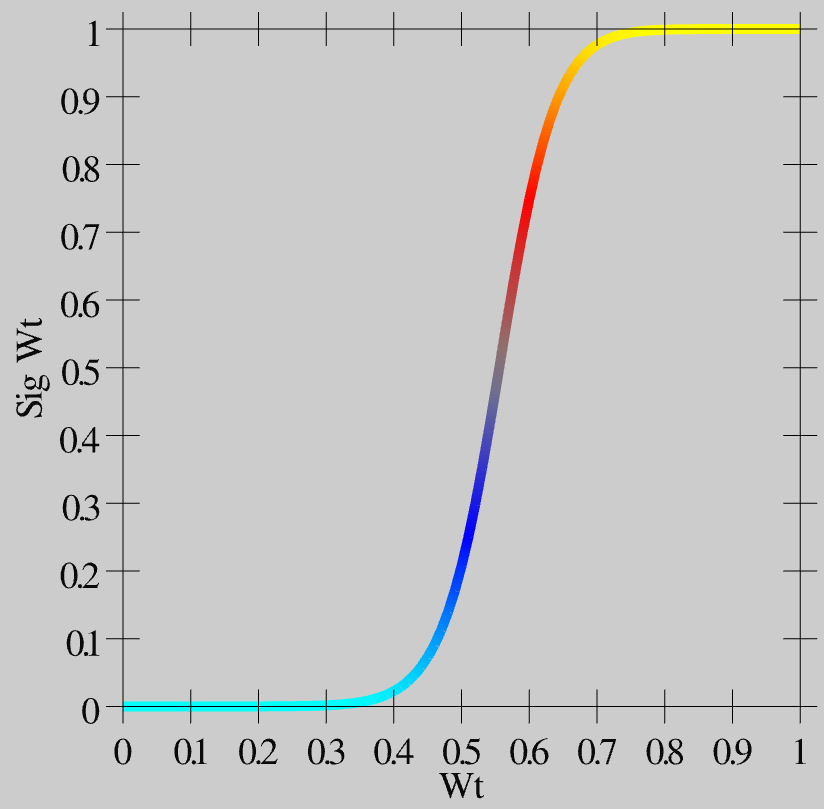
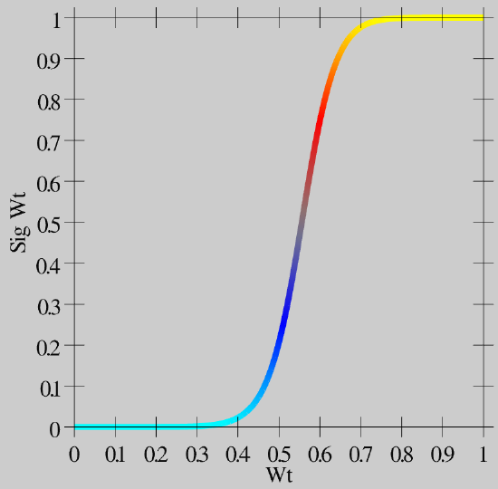
The exponential approach function works well at keeping weights bounded in a graded way (much better than simply clipping weight values at the bounds, which loses all the signal for saturated weights), but it also creates a strong tendency for weights to hang out in the middle of the range, around .5. This creates problems because then neurons don't have sufficiently distinct responses to different input patterns, and then the inhibitory competition breaks down (many neurons become weakly activated), which then interferes with the positive feedback loop that is essential for learning, etc. To counteract these problems, while maintaining the exponential bounding, we introduce a contrast enhancement function on the weights:

• \(\hat{w}=\frac{1}{1+\left(\frac{w}{\theta(1-w)}\right)^{-\gamma}}\)

As you can see in Figure 4.11, this function creates greater contrast for weight values around this .5 central value -- they get pushed up or down to the extremes. This contrast-enhanced weight value is then used for communication among the neurons, and is what shows up as the wt value in the simulator.

Figure \(4.11\): Weight contrast enhancement function, gain (gamma) = 6, offset (theta) = 1.25.

Biologically, we think of the plain weight value w, which is involved in the learning functions, as an internal variable that accurately tracks the statistics of the learning functions, while the contrast-enhanced weight value is the actual synaptic efficacy value that you measure and observe as the strength of interaction among neurons. Thus, the plain w value may correspond to the phosphorylation state of CAMKII or some other appropriate internal value that mediates synaptic plasticity.

Finally, see Implementational Details for a few implementational details about the way that the time averages are computed, which don't affect anything conceptually, but if you really want to know exactly what is going on..