3.4: Bidirectional Excitatory Dynamics and Attractors
- Page ID
- 12576
The feedforward flow of excitation through multiple layers of the neocortex can make us intelligent, but the feedback flow of excitation in the opposite direction is what makes us robust, flexible, and adaptive. Without this feedback pathway, the system can only respond on the basis of whatever happens to drive the system most strongly in the feedforward, bottom-up flow of information. But often our first impression is wrong, or at least incomplete. In the "searching for a friend" example from the introduction, we might not get sufficiently detailed information from scanning the crowd to drive the appropriate representation of the person. Top-down activation flow can help focus us on relevant perceptual information that we can spot (like the red coat). As this information interacts with the bottom-up information coming in as we scan the crowd, our brains suddenly converge on the right answer: There's my friend, in the red coat!

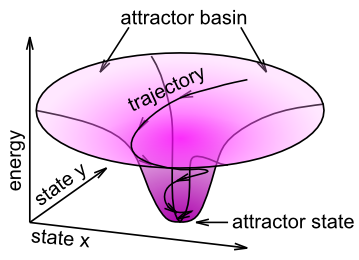
The overall process of converging on a good internal representation given a noisy, weak or otherwise ambiguous input can be summarized in terms of attractor dynamics (Figure 3.14). An attractor is a concept from dynamical systems theory, representing a stable configuration that a dynamical system will tend to gravitate toward. A familiar example of attractor dynamics is the coin gravity well, often found in science museums. You roll your coin down a slot at the top of the device, and it rolls out around the rim of an upside-down bell-shaped "gravity well". It keeps orbiting around the central hole of this well, but every revolution brings it closer to the "attractor" state in the middle. No matter where you start your coin, it will always get sucked into the same final state. This is the key idea behind an attractor: many different inputs all get sucked into the same final state. If the attractor dynamic is successful, then this final state should be the correct categorization of the input pattern.

There are many different instances where bidirectional excitatory dynamics are evident:
- Top-down imagery -- I can ask you to imagine what a purple hippopotamus looks like, and you can probably do it pretty well, even if you've never seen one before. Via top-down excitatory connections, high-level verbal inputs can drive corresponding visual representations. For example, imagining the locations of different things in your home or apartment produces reaction times that mirror the actual spatial distances between those objects -- we seem to be using a real spatial/visual representation in our imagery. (See Imagery Debate for brief discussion of a long debate in the literature on this topic).
- Top-down ambiguity resolution -- Many stimuli are ambiguous without further top-down constraints. For example, if you've never seen Figure 3.15 before, you probably won't be able to find the Dalmatian dog in it. But now that you've read that clue, your top-down semantic knowledge about what a dalmatian looks like can help your attractor dynamics converge on a coherent view of the scene.
- Pattern completion -- If I ask you "what did you have for dinner last night", this partial input cue can partially excite the appropriate memory representation in your brain (likely in the hippocampus), but you need a bidirectional excitatory dynamic to enable this partial excitation to reverberate through the memory circuits and fill in the missing parts of the full memory trace. This reverberatory process is just like the coin orbiting around the gravity well -- different neurons get activated and inhibited as the system "orbits" around the correct memory trace, eventually converging on the full correct memory trace (or not!). Sometimes, in so-called tip of the tongue states, the memory you're trying to retrieve is just beyond grasp, and the system cannot quite converge into its attractor state. Man, that can be frustrating! Usually you try everything to get into that final attractor. We don't like to be in an unresolved state for very long.
Energy and Harmony
There is a mathematical way to capture something like the vertical axis in the attractor figure (Figure 3.14), which in the physical terms of a gravity well is potential energy. Perhaps not surprisingly, this measure is called energy and it was developed by a physicist named John Hopfield. He showed that local updating of unit activation states ends up reducing a global energy measure, much in the same way that local motion of the coin in the gravity well reduces its overall potential energy. Another physicist, Paul Smolensky, developed an alternative framework with the sign reversed, where local updating of unit activation states increases global Harmony. That sounds nice, doesn't it? To see the mathematical details, see Energy and Harmony. We don't actually need these equations to run our models, and the basic intuition for what they tell us is captured by the notion of an attractor, so we won't spend any more time on this idea in this main chapter.
Explorations
See Face Categorization (Part II) for an exploration of how top-down and bottom-up processing interact to produce imagery and help resolve ambiguous inputs (partially occluded faces). These additional simulations provide further elaboration of bidirectional computation:
- Cats and Dogs -- fun example of attractor dynamics in a simple semantic network.
- Necker Cube -- another fun example of attractor dynamics, showing also the important role of noise, and neural fatigue.


