
6.4: Invariant Object Recognition in the "What" Pathway
- Page ID
- 12599

Object recognition is the defining function of the ventral "what" pathway of visual processing: identifying what you are looking at. Neurons in the inferotemporal (IT) cortex can detect whole objects, such as faces, cars, etc, over a large region of visual space. This spatial invariance (where the neural response remains the same or invariant over spatial locations) is critical for effective behavior in the world -- objects can show up in all different locations, and we need to recognize them regardless of where they appear. Achieving this outcome is a very challenging process, one which has stumped artificial intelligence (AI) researchers for a long time -- in the early days of AI, the 1960's, it was optimistically thought that object recognition could be solved as a summer research project, and 50 years later we are making a lot of progress, but it remains unsolved in the sense that people are still much better than our models. Because our brains do object recognition effortlessly all the time, we do not really appreciate how hard of a problem it is.
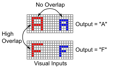
The reason object recognition is so hard is that there can often be no overlap at all among visual inputs of the same object in different locations (sizes, rotations, colors, etc), while there can be high levels of overlap among different objects in the same location (Figure 6.10). Therefore, you cannot rely on the bottom-up visual similarity structure -- instead it often works directly against the desired output categorization of these stimuli. As we saw in the Learning Chapter, successful learning in this situation requires error-driven learning, because self-organizing learning tends to be strongly driven by the input similarity structure.


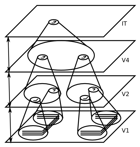
The most successful approach to the object recognition problem, which was advocated initially in a model by Fukushima (1980), is to incrementally solve two problems over a hierarchically organized sequence of layers (Figure 6.11, Figure 6.12):
- The invariance problem, by having each layer integrate over a range of locations (and sizes, rotations, etc) for the features in the previous layer, such that neurons become increasingly invariant as one moves up the hierarchy.
- The pattern discrimination problem (distinguishing an A from an F, for example), by having each layer build up more complex combinations of feature detectors, as a result of detecting combinations of the features present in the previous layer, such that neurons are better able to discriminate even similar input patterns as one moves up the hierarchy.
The critical insight from these models is that breaking these two problems down into incremental, hierarchical steps enables the system to solve both problems without one causing trouble for the other. For example, if you had a simple fully invariant vertical line detector that responded to a vertical line in any location, it would be impossible to know what spatial relationship this line has with other input features, and this relationship information is critical for distinguishing different objects (e.g., a T and L differ only in the relationship of the two line elements). So you cannot solve the invariance problem in one initial pass, and then try to solve the pattern discrimination problem on top of that. They must be interleaved, in an incremental fashion. Similarly, it would be completely impractical to attempt to recognize highly complex object patterns at each possible location in the visual input, and then just do spatial invariance integration over locations after that. There are way too many different objects to discriminate, and you'd have to learn about them anew in each different visual location. It is much more practical to incrementally build up a "part library" of visual features that are increasingly invariant, so that you can learn about complex objects only toward the top of the hierarchy, in a way that is already spatially invariant and thus only needs to be learned once.

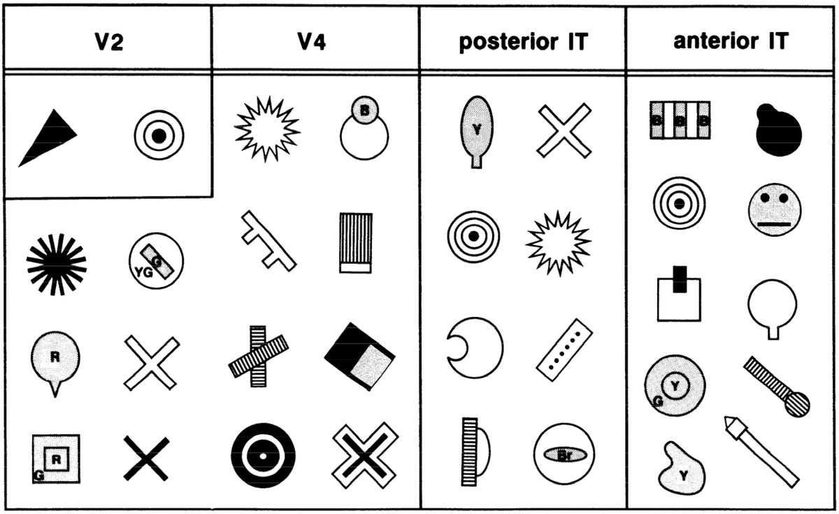
In a satisfying convergence of top-down computational motivation and bottom-up neuroscience data, this incremental, hierarchical solution provides a nice fit to the known properties of the visual areas along the ventral what pathway (V1, V2, V4, IT). Figure 6.13 summarizes neural recordings from these areas in the macaque monkey, and shows that neurons increase in the complexity of the stimuli that drive their responding, and the size of the receptive field over which they exhibit an invariant response to these stimuli, as one proceeds up the hierarchy of areas. Figure 6.14 shows example complex stimuli that evoked maximal responding in each of these areas, to give a sense of what kind of complex feature conjunctions these neurons can detect.

See Ventral Path Data for a more detailed discussion of the data on neural responses to visual shape features in these ventral pathways, including several more data figures. There are some interesting subtleties and controversies in this literature, but the main conclusions presented here still hold.
Exploration of Object Recognition

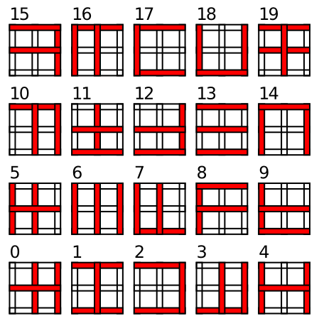
Go to Objrec for the computational model of object recognition, which demonstrates the incremental hierarchical solution to the object recognition problem. We use a simplified set of "objects" (Figure 6.15) composed from vertical and horizontal line elements. This simplified set of visual features allows us to better understand how the model works, and also enables testing generalization to novel objects composed from these same sets of features. You will see that the model learns simpler combinations of line elements in area V4, and more complex combinations of features in IT, which are also invariant over the full receptive field. These IT representations are not identical to entire objects -- instead they represent an invariant distributed code for objects in terms of their constituent features. The generalization test shows how this distributed code can support rapid learning of new objects, as long as they share this set of features. Although they are likely much more complex and less well defined, it seems that a similar such vocabulary of visual shape features are learned in primate IT representations.