
1.4: Introduction to 2 x 2 Tables, Epidemiologic Study Design, and Measures of Association
- Page ID
- 38517

\( \newcommand{\vecs}[1]{\overset { \scriptstyle \rightharpoonup} {\mathbf{#1}} } \)
\( \newcommand{\vecd}[1]{\overset{-\!-\!\rightharpoonup}{\vphantom{a}\smash {#1}}} \)
\( \newcommand{\dsum}{\displaystyle\sum\limits} \)
\( \newcommand{\dint}{\displaystyle\int\limits} \)
\( \newcommand{\dlim}{\displaystyle\lim\limits} \)
\( \newcommand{\id}{\mathrm{id}}\) \( \newcommand{\Span}{\mathrm{span}}\)
( \newcommand{\kernel}{\mathrm{null}\,}\) \( \newcommand{\range}{\mathrm{range}\,}\)
\( \newcommand{\RealPart}{\mathrm{Re}}\) \( \newcommand{\ImaginaryPart}{\mathrm{Im}}\)
\( \newcommand{\Argument}{\mathrm{Arg}}\) \( \newcommand{\norm}[1]{\| #1 \|}\)
\( \newcommand{\inner}[2]{\langle #1, #2 \rangle}\)
\( \newcommand{\Span}{\mathrm{span}}\)
\( \newcommand{\id}{\mathrm{id}}\)
\( \newcommand{\Span}{\mathrm{span}}\)
\( \newcommand{\kernel}{\mathrm{null}\,}\)
\( \newcommand{\range}{\mathrm{range}\,}\)
\( \newcommand{\RealPart}{\mathrm{Re}}\)
\( \newcommand{\ImaginaryPart}{\mathrm{Im}}\)
\( \newcommand{\Argument}{\mathrm{Arg}}\)
\( \newcommand{\norm}[1]{\| #1 \|}\)
\( \newcommand{\inner}[2]{\langle #1, #2 \rangle}\)
\( \newcommand{\Span}{\mathrm{span}}\) \( \newcommand{\AA}{\unicode[.8,0]{x212B}}\)
\( \newcommand{\vectorA}[1]{\vec{#1}} % arrow\)
\( \newcommand{\vectorAt}[1]{\vec{\text{#1}}} % arrow\)
\( \newcommand{\vectorB}[1]{\overset { \scriptstyle \rightharpoonup} {\mathbf{#1}} } \)
\( \newcommand{\vectorC}[1]{\textbf{#1}} \)
\( \newcommand{\vectorD}[1]{\overrightarrow{#1}} \)
\( \newcommand{\vectorDt}[1]{\overrightarrow{\text{#1}}} \)
\( \newcommand{\vectE}[1]{\overset{-\!-\!\rightharpoonup}{\vphantom{a}\smash{\mathbf {#1}}}} \)
\( \newcommand{\vecs}[1]{\overset { \scriptstyle \rightharpoonup} {\mathbf{#1}} } \)
\(\newcommand{\longvect}{\overrightarrow}\)
\( \newcommand{\vecd}[1]{\overset{-\!-\!\rightharpoonup}{\vphantom{a}\smash {#1}}} \)
\(\newcommand{\avec}{\mathbf a}\) \(\newcommand{\bvec}{\mathbf b}\) \(\newcommand{\cvec}{\mathbf c}\) \(\newcommand{\dvec}{\mathbf d}\) \(\newcommand{\dtil}{\widetilde{\mathbf d}}\) \(\newcommand{\evec}{\mathbf e}\) \(\newcommand{\fvec}{\mathbf f}\) \(\newcommand{\nvec}{\mathbf n}\) \(\newcommand{\pvec}{\mathbf p}\) \(\newcommand{\qvec}{\mathbf q}\) \(\newcommand{\svec}{\mathbf s}\) \(\newcommand{\tvec}{\mathbf t}\) \(\newcommand{\uvec}{\mathbf u}\) \(\newcommand{\vvec}{\mathbf v}\) \(\newcommand{\wvec}{\mathbf w}\) \(\newcommand{\xvec}{\mathbf x}\) \(\newcommand{\yvec}{\mathbf y}\) \(\newcommand{\zvec}{\mathbf z}\) \(\newcommand{\rvec}{\mathbf r}\) \(\newcommand{\mvec}{\mathbf m}\) \(\newcommand{\zerovec}{\mathbf 0}\) \(\newcommand{\onevec}{\mathbf 1}\) \(\newcommand{\real}{\mathbb R}\) \(\newcommand{\twovec}[2]{\left[\begin{array}{r}#1 \\ #2 \end{array}\right]}\) \(\newcommand{\ctwovec}[2]{\left[\begin{array}{c}#1 \\ #2 \end{array}\right]}\) \(\newcommand{\threevec}[3]{\left[\begin{array}{r}#1 \\ #2 \\ #3 \end{array}\right]}\) \(\newcommand{\cthreevec}[3]{\left[\begin{array}{c}#1 \\ #2 \\ #3 \end{array}\right]}\) \(\newcommand{\fourvec}[4]{\left[\begin{array}{r}#1 \\ #2 \\ #3 \\ #4 \end{array}\right]}\) \(\newcommand{\cfourvec}[4]{\left[\begin{array}{c}#1 \\ #2 \\ #3 \\ #4 \end{array}\right]}\) \(\newcommand{\fivevec}[5]{\left[\begin{array}{r}#1 \\ #2 \\ #3 \\ #4 \\ #5 \\ \end{array}\right]}\) \(\newcommand{\cfivevec}[5]{\left[\begin{array}{c}#1 \\ #2 \\ #3 \\ #4 \\ #5 \\ \end{array}\right]}\) \(\newcommand{\mattwo}[4]{\left[\begin{array}{rr}#1 \amp #2 \\ #3 \amp #4 \\ \end{array}\right]}\) \(\newcommand{\laspan}[1]{\text{Span}\{#1\}}\) \(\newcommand{\bcal}{\cal B}\) \(\newcommand{\ccal}{\cal C}\) \(\newcommand{\scal}{\cal S}\) \(\newcommand{\wcal}{\cal W}\) \(\newcommand{\ecal}{\cal E}\) \(\newcommand{\coords}[2]{\left\{#1\right\}_{#2}}\) \(\newcommand{\gray}[1]{\color{gray}{#1}}\) \(\newcommand{\lgray}[1]{\color{lightgray}{#1}}\) \(\newcommand{\rank}{\operatorname{rank}}\) \(\newcommand{\row}{\text{Row}}\) \(\newcommand{\col}{\text{Col}}\) \(\renewcommand{\row}{\text{Row}}\) \(\newcommand{\nul}{\text{Nul}}\) \(\newcommand{\var}{\text{Var}}\) \(\newcommand{\corr}{\text{corr}}\) \(\newcommand{\len}[1]{\left|#1\right|}\) \(\newcommand{\bbar}{\overline{\bvec}}\) \(\newcommand{\bhat}{\widehat{\bvec}}\) \(\newcommand{\bperp}{\bvec^\perp}\) \(\newcommand{\xhat}{\widehat{\xvec}}\) \(\newcommand{\vhat}{\widehat{\vvec}}\) \(\newcommand{\uhat}{\widehat{\uvec}}\) \(\newcommand{\what}{\widehat{\wvec}}\) \(\newcommand{\Sighat}{\widehat{\Sigma}}\) \(\newcommand{\lt}{<}\) \(\newcommand{\gt}{>}\) \(\newcommand{\amp}{&}\) \(\definecolor{fillinmathshade}{gray}{0.9}\)Learning Objectives
After reading this chapter, you will be able to do the following:
- Interpret data found in a 2 x 2 table
- Compare and contrast the 4 most common types of epidemiologic studies: cohort studies, randomized controlled trials, case-control studies, and cross-sectional studies
- Calculate and interpret relative measures of association (risk ratios, rate ratios, odds ratios)
- Explain which measures are preferred for which study designs and why
- Discuss the differences between absolute and relative measures of association
In epidemiology, we are often concerned with the degree to which a particular exposure might cause (or prevent) a particular disease. As detailed later in chapter 10, it is difficult to claim causal effects from a single epidemiologic study; therefore, we say instead that exposures and diseases are (or are not) statistically associated. This means that the exposure is disproportionately distributed between individuals with and without the disease. The degree to which exposures and health outcomes are associated is conveyed through a measure of association. Which measure of association to choose depends on whether you are working with incidence or prevalence data, which in turn depends on the type of study design used. This chapter will therefore provide a brief outline of common epidemiologic study designs interwoven with a discussion of the appropriate measure(s) of association for each. In chapter 9, we will return to study designs for a more in-depth discussion of their strengths and weaknesses.
Necessary First Step: 2 x 2 Notation
Before getting into study designs and measures of association, it is important to understand the notation used in epidemiology to convey exposure and disease data: the 2 x 2 table. A 2 x 2 table (or two-by-two table) is a compact summary of data for 2 variables from a study—namely, the exposure and the health outcome. Say we do a 10-person study on smoking and hypertension, and collect the following data, where Y indicates yes and N indicates no:
| Participant # | Smoker? | Hypertension? |
|---|---|---|
| 1 | Y | Y |
| 2 | Y | N |
| 3 | Y | Y |
| 4 | Y | Y |
| 5 | N | N |
| 6 | N | Y |
| 7 | N | N |
| 8 | N | N |
| 9 | N | Y |
| 10 | N | N |
You can see that we have 4 smokers, 6 nonsmokers, 5 individuals with hypertension, and 5 without. In this example, smoking is the exposure and hypertension is the health outcome, so we say that the 4 smokers are “exposed” (E+), the 6 nonsmokers are “unexposed” (E−), the 5 people with hypertension are “diseased” (D+), and the 5 people without hypertension are “nondiseased” (D−). This information can be organized into a 2 × 2 table:
| D+ | D- | |
|---|---|---|
| E+ | 3 | 1 |
| E- | 2 | 4 |
The 2 × 2 table summarizes the information from the longer table above so that you can quickly see that 3 individuals were both exposed and diseased (persons 1, 3, and 4); one individual was exposed but not diseased (person 2); two individuals were unexposed but diseased (persons 6 and 9); and the remaining 4 individuals were neither exposed nor diseased (persons 5, 7, 8, and 10). Though it does not really matter whether exposure or disease is placed on the left or across the top of a 2 × 2 table, the convention in epidemiology is to have exposure on the left and disease across the top.
When discussing 2 x 2 tables, epidemiologists use the following shorthand to refer to specific cells:
| D+ | D- | |
|---|---|---|
| E+ | A | B |
| E- | C | D |
It is often helpful to calculate the margin totals for a 2 x 2 table:
| D+ | D- | Total | |
| E+ | 3 | 1 | 4 |
| E- | 2 | 4 | 6 |
| Total | 5 | 5 | 10 |
Or:
| D+ | D- | Total | |
| E+ | A | B | A+B |
| E- | C | D | C+D |
| Total | A+C | B+D | A+B+C+D |
The margin totals are sometimes helpful when calculating various measures of association (and to check yourself against the original data).
Continuous versus Categorical Variables
Continuous variables are things such as age or height, where the possible values for a given person are infinite, or close to it. Categorical variables are things such as religion or favorite color, where there is a discrete list of possible answers. Dichotomous variables are a special case of categorical variable where there are only 2 possible answers. It is possible to dichotomize a continuous variable—if you have an “age” variable, you could split it into “old” and “young.” However, is it not always advisable to do this because a lot of information is lost. Furthermore, how does one decide where to dichotomize? Does “old” start at 40, or 65? Epidemiologists usually prefer to leave continuous variables continuous to avoid having to make these judgment calls.
Nonetheless, having dichotomous variables (a person is either exposed or not, either diseased or not) makes the math much easier to understand. For the purposes of this book, then, we will assume that all exposure and disease data can be meaningfully dichotomized and placed into 2×2 tables.
Studies That Use Incidence Data
Cohorts
There are 4 types of epidemiologic studies that will be covered in this book,[1] two of which collect incidence data: prospective cohort studies and randomized controlled trials. Since these study designs use incidence data, we instantly know 3 things about these study types. One, we are looking for new cases of disease. Two, there is thus some longitudinal follow-up that must occur to allow for these new cases to develop. Three, we must start with those who were at risk (i.e., without the disease or health outcome) as our baseline.
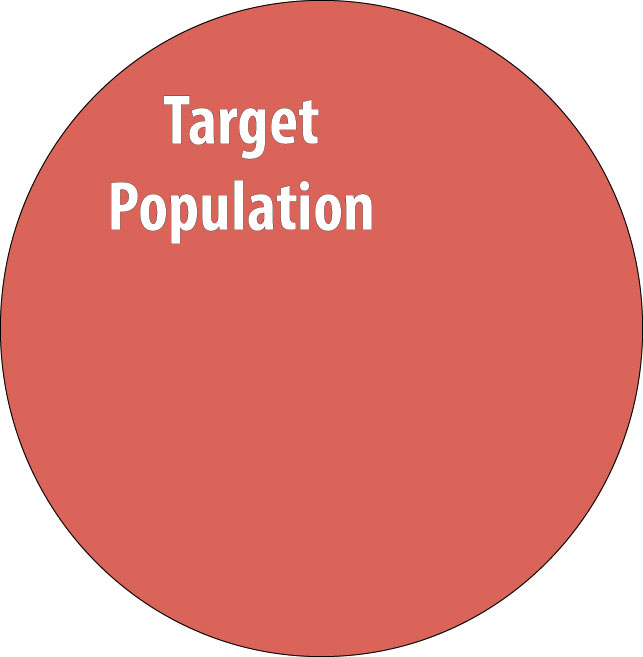
The procedure for a prospective cohort study (hereafter referred to as just a “cohort study,” though see the inset box on retrospective cohort studies later in this chapter) begins with the target population, which contains both diseased and non-diseased individuals:
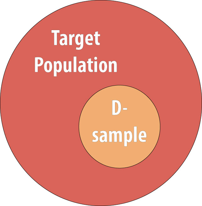
As discussed in chapter 1, we rarely conduct studies on entire populations because they are too big for it to be logistically feasible to study everyone in the population. Therefore we draw a sample and perform the study with the individuals in the sample. For a cohort study, since we will be calculating incidence, we must start with individuals who are at risk of the outcome. We thus draw a non-diseased sample from the target population:
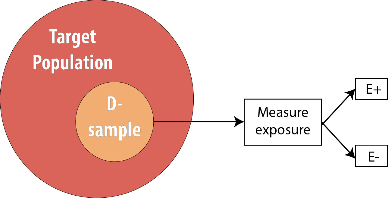
The next step is to assess the exposure status of the individuals in our sample and determine whether they are exposed or not:
After assessing which participants were exposed, our 2 x 2 table (using the 10-person smoking/HTN data example from above) would look like this:
| D+ | D- | Total | |
| E+ | 0 | 4 | 4 |
| E- | 0 | 6 | 6 |
| Total | 0 | 10 | 10 |
By definition, at the beginning of a cohort study, everyone is still at risk of developing the disease, and therefore there are no individuals in the D+ column. In this hypothetical example, based on the data above, we will observe 5 cases of incident hypertension as the study progresses–but at the beginning, none of these cases have yet occurred.
We then follow the participants in our study for some length of time and observe incident cases as they arise.
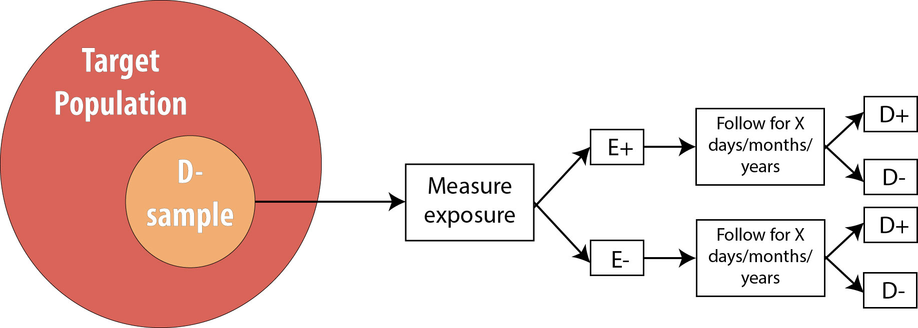
As mentioned in chapter 2, the length of follow-up varies depending on the disease process in question. For a research question regarding childhood exposure and late-onset cancer, the length of follow-up would be decades. For an infectious disease outbreak, the length of follow-up might be a matter of days or even hours, depending on the incubation period of the particular disease.
Assuming we are calculating incidence proportions (which use the number of people at risk in the denominator) in our cohort, our 2 × 2 table at the end of the smoking/HTN study would look like this:
| D+ | D- | Total | |
| E+ | 3 | 1 | 4 |
| E- | 2 | 4 | 6 |
| Total | 5 | 5 | 10 |
It is important to recognize that when epidemiologists talk about a 2 × 2 table from a cohort study, they mean the 2 × 2 table at the end of the study—the 2 × 2 table from the beginning was much less interesting, as the D+ column was empty!
From this 2 × 2 table, we can calculate a number of useful measures, detailed below.
Example \(\PageIndex{1}\): Calculating the Risk Ratio from the Hypothetical Smoking/Hypertension Cohort Study
We can start by calculating the overall incidence of disease in our sample (assume that our smoking/HTN study included 10 years of follow-up):
\[\text { Incidence proportion = population at risk at baseline }=\frac{5}{10}\]
This is 50 cases per 100 people in 10 years
Using ABCD notation for a 2 x 2 table, the formula for the overall incidence proportion is:
We can also calculate the incidence only among exposed individuals:
\[I_{E+}=\frac{A}{(A+B)}=\frac{3}{4}=75 \text { per } 100 \text { in } 10 \text { years }\]
Likewise, we can calculate the incidence only among unexposed individuals:
\[\mathrm{I}_{\mathrm{E}-}=\frac{C}{(C+D)}=\frac{2}{6}=33 \text { per } 100 \text { in } 10 \text { years }\]
Recall that our original goal with the cohort study was to see whether exposure is associated with disease. We thus need to compare the IE+ to the IE-. The most common way of doing this is to calculate their combined ratio:
\[\text { Risk Ratio }=\frac{I_{E+}}{I_{E-}}=\frac{75 \text { per } 100 \text { in } 10 \text { years }}{33 \text { per } 100 \text { in } 10 \text { years }}=2.27\]
Using ABCD notation, the formula for RR is:
\[RR=\frac{\frac{A}{(A+B)}}{\frac{C}{(C+D)}}\]
Note that risk ratios (RR) have no units, because the time-dependent units for the 2 incidences cancel out.
If the RR is greater than 1, it means that we observed more disease in the exposed group than in the unexposed group. Likewise, if the RR is less than 1, it means that we observed less disease in the exposed group than in the unexposed group. If we assume causality, an exposure with an RR < 1 is preventing disease, and an exposure with an RR > 1 is causing disease. The null value for a risk ratio is 1.0, which would mean that there was no observed association between exposure and disease. You can see how this would be the case—if the incidence was identical in the exposed and unexposed groups, then the RR would be 1, since x divided by x is 1.
Because the null value is 1.0, one must be careful if using the words higher or lower when interpreting RRs. For instance, an RR of 2.0 means that the disease is twice as common, or twice as high, in the exposed compared to the unexposed—not that it is 2 times more common, or 2 times higher, which would be an RR of 3.0 (since the null value is 1, not 0). If you do not see the distinction between these, don’t sweat it—just memorize and use the template sentence below, and your interpretation will be correct.
The correct interpretation of an RR is:
Using our smoking/HTN example:
The key phrase is times as high; with it, the template sentence works regardless of whether the RR is above or below 1. For an RR of 0.5, saying “0.5 times as high” means that you multiply the risk in the unexposed by 0.5 to get the risk in the exposed, yielding a lower incidence in the exposed—as one expects with an RR < 1.
If our cohort study instead used a person-time approach, the 2 x 2 table at the end of the study would have a column for sum of the person-time at risk (PTAR):
| D+ | D- | Total | Σ PTAR | |
| E+ | 3 | 1 | 4 | 27.3 PY |
| E- | 2 | 4 | 6 | 52.9 PY |
| Total | 5 | 5 | 10 | 80.2 PY |
Example \(\PageIndex{2}\): Calculating the Rate Ratio from the Hypothetical Smoking/Hypertension Cohort Study
Using a person-time denominator, the incidence rate for the overall study is:
Likewise, the incidence rate among exposed persons is:
And the incidence among unexposed persons is:
We again take the ratio of incidence in the exposed to incidence in the unexposed, this time calculating a rate ratio (also abbreviated RR):
As when using incidence proportions, the units cancel out, and we are left with just a number.
The interpretation is the same as it would be for the risk ratio; one just needs to substitute the word rate for the word risk:
Notice that the interpretation sentence still includes the duration of the study, even though some individuals (the 4 who developed hypertension) were censored before that time. This is because knowing how long people were followed for (and thus given time to develop disease) is still important when interpreting the findings. As discussed in chapter 2, 100 years of person-time can be accumulated in any number of different ways; knowing that the duration of the study was 10 years (rather than 1 year or 50 years) might make a difference in terms of how (or if) one applies the findings in practice.
“Relative Risk”
Both the risk ratio and the rate ratio are abbreviated RR. This abbreviation (and the risk ratio and/or rate ratio) is often referred to by epidemiologists as relative risk. This is an example of inconsistent lexicon in the field of epidemiology; in this book, I use risk ratio and rate ratio separately (rather than relative risk as an umbrella term) because it is helpful, in my opinion, to distinguish between studies using the population at risk vs. those using a person-time at risk approach. Regardless, a measure of association called RR is always calculated as incidence in the exposed divided by incidence in the unexposed.
Retrospective Cohort Studies
Throughout this book, I will focus on prospective cohort studies. One can also conduct a retrospective cohort study, mentioned here because public health and clinical practitioners will encounter retrospective cohort studies in the literature. In theory, a retrospective cohort study is conducted exactly like a prospective cohort study: one begins with a non-diseased sample from the target population, determines who was exposed, and “follows” the sample for x days/months/years, looking for incident cases of disease. The difference is that, for a retrospective cohort study, all this has already happened, and one reconstructs this information using existing records. The most common way to do retrospective cohort studies is by using employment records (which often have job descriptions useful for surmising exposure—for instance, the floor manager was probably exposed to whatever chemicals were on the factory floor, whereas human resource officers probably were not), medical records, or other administrative datasets (e.g., military records).
Continuing with our smoking/HTN 10-year cohort example, one might do a retrospective cohort using medical records as follows:
- Go back to all the records from 10 years ago and determine who already had hypertension (these people are not at risk and are therefore not eligible) or otherwise does not meet the sample inclusion criteria
- Determine, among those at risk 10 years ago, which individuals were smokers
- Determine which members of the sample then developed hypertension during the intervening 10 years
Retrospective cohorts are analyzed just like prospective cohorts—that is, by calculating rate ratios or risk ratios. However, for beginning epidemiology students, retrospective cohorts are often confused with case-control studies; therefore we will focus exclusively on prospective cohorts for the remainder of this book. (Indeed, occasionally even seasoned scientists are confused about the difference!)i
Randomized Controlled Trials
The procedure for a randomized controlled trial (RCT) is exactly the same as the procedure for a prospective cohort, with one exception: instead of allowing participants to self-select into “exposed” and “unexposed” groups, the investigator in an RCT randomly assigns some participants (usually half) to “exposed” and the other half to “unexposed.” In other words, exposure status is determined entirely by chance. This is the type of study required by the Food and Drug Administration for approval of new drugs: half of the participants in the study are randomly assigned to the new drug and half to the old drug (or to a placebo, if the drug is intended to treat something previously untreatable). The diagram for an RCT is as follows:
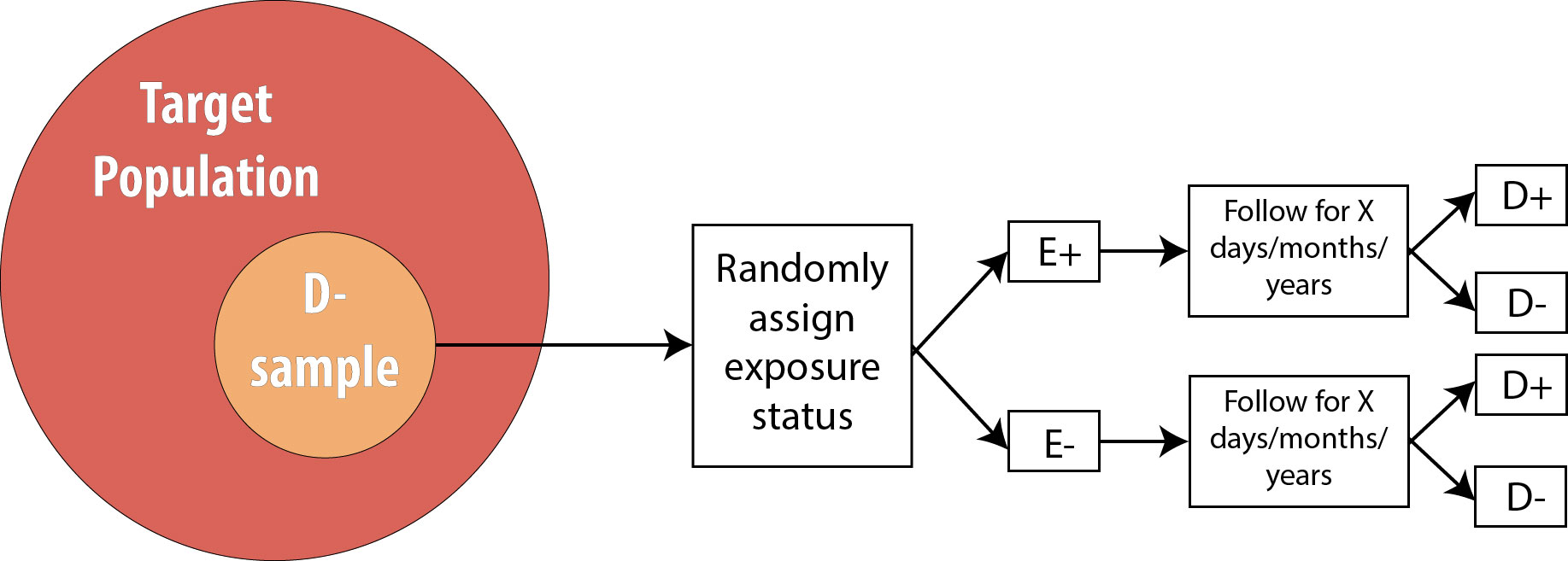
Note that the only difference between an RCT and a prospective cohort is the first box: instead of measuring existing exposures, we now tell people whether they will be exposed or not. We are still measuring incident disease, and we are therefore still calculating either the risk ratio or the rate ratio.
Observational versus Experimental Studies
Cohort studies are a subclass of observational studies, meaning the researcher is merely observing what happens in real life—people in the study self-select into being exposed or not depending on their personal preferences and life circumstances. The researcher then measures and records a given person’s level of exposure. Cross-sectional and case-control studies are also observational. Randomized controlled trials, on the other hand, are experimental studies—the researcher is conducting an experiment that involves telling people whether they will be exposed to a condition or not (e.g., to a new drug).
Studies That Use Prevalence Data
Following participants while waiting for incident cases of disease is expensive and time-consuming. Often, epidemiologists need a faster (and cheaper) answer to their question about a particular exposure/disease combination. One might instead take advantage of prevalent cases of disease, which by definition have already occurred and therefore require no wait. There are 2 such designs that I will cover: cross-sectional studies and case-control studies. For both of these, since we are not using incident cases, we cannot calculate the RR, because we have no data on incidence. We instead calculate the odds ratio (OR).
Cross-sectional
Cross-sectional studies are often referred to as snapshot or prevalence studies: one takes a “snapshot” at a particular point in time, determining who is exposed and who is diseased simultaneously. The following is a visual:
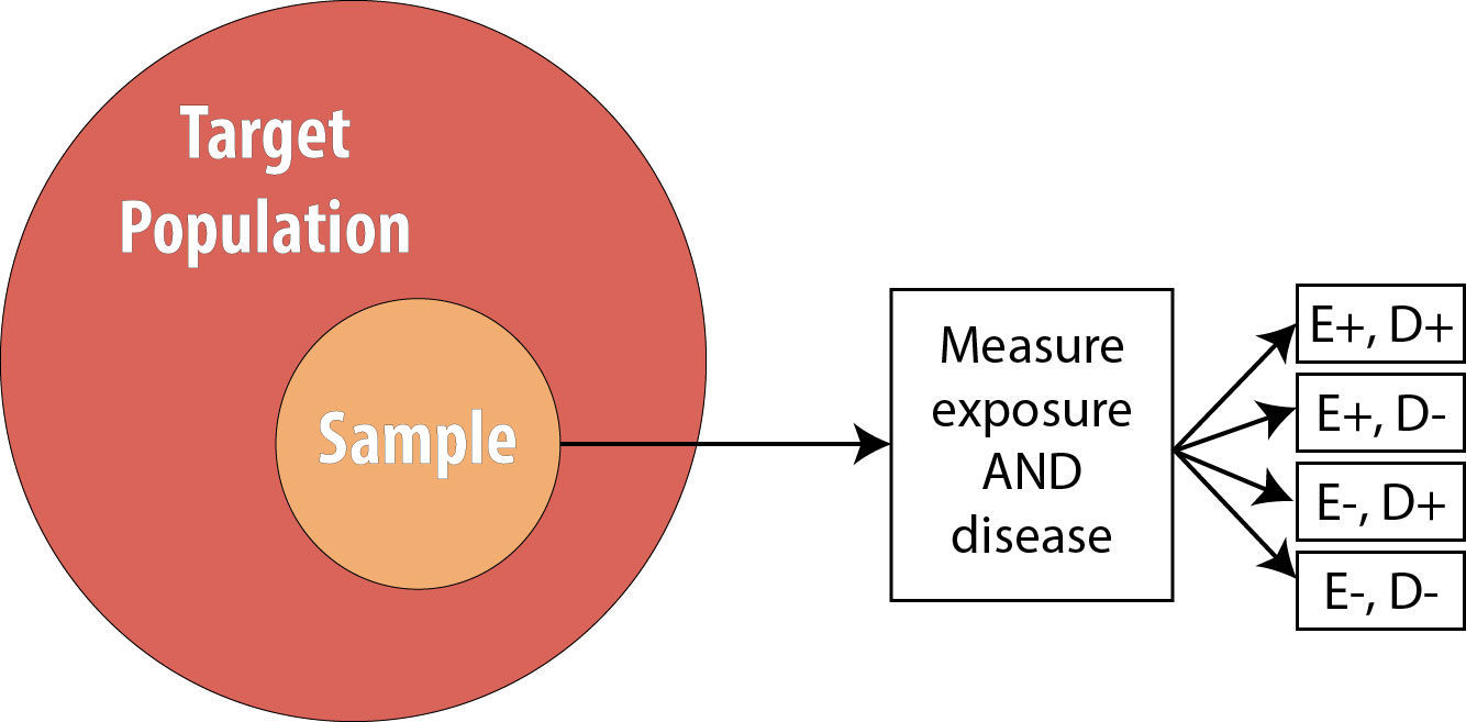
Note that the sample is now no longer composed entirely of those at risk because we are using prevalent cases—thus by definition, some proportion of the sample will be diseased at baseline. As mentioned, we cannot calculate the RR in this scenario, so instead we calculate the OR.
Example \(\PageIndex{3}\): Calculating the Odds Ratio from the Hypothetical Smoking/Hypertension Cross-Sectional Study
The formula for OR for a cross-sectional study is:
\[\mathrm{OR}=\frac{\text { odds of disease in the exposed group }}{\text { odds of disease in the unexposed group }} \nonumber\]
The odds of an event is defined statistically as the number of people who experienced an event divided by the number of people who did not experience it. Using 2 × 2 notation, the formula for OR is:
\[\mathrm{OR}=\frac{\frac{A}{B}}{\frac{C}{D}}=\frac{A D}{B C} \nonumber\]
For our smoking/HTN example, if we assume those data came from a cross-sectional study, the OR would be:
\[\mathrm{OR}=\frac{\frac{3}{1}}{\frac{2}{4}}=\frac{3 * 4}{2 * 1}=6.0 \nonumber\]
Again there are no units.
The interpretation of an OR is the same as that of an RR, with the word odds substituted for risk:
Note that we now no longer mention time, as these data came from a cross-sectional study, which does not involve time. As with interpretation of RRs, ORs greater than 1 mean the exposure is more common among diseased, and ORs less than 1 mean the exposure is less common among diseased. The null value is again 1.0.
For 2 x 2 tables from cross-sectional studies, one can additionally calculate the overall prevalence of disease as
Finally, some authors will refer to the OR in a cross-sectional study as the prevalence odds ratio—presumably, just as a reminder that cross-sectional studies are conducted on prevalent cases. The calculation of such a measure is exactly the same as the OR as presented above.
OR versus RR
As you can see from the (hypothetical) example data in this chapter, the OR will always be further from the null value than the RR. The more common the disease, the more this is true. If the disease has a prevalence of about 5% or less, then the OR does provide a close approximation of the RR; however, as the disease in question becomes more common (as in this example, with a hypertension prevalence of 40%), the OR deviates further and further from the RR.
Occasionally, you will see a cohort study (or very rarely, an RCT) that reports the OR instead of the RR. Technically this is not correct, because cohorts and RCTs use incident cases, so the best choice for a measure of association is the RR. However, one common statistical modeling technique—logistic regression—automatically calculates ORs. While it is possible to back-calculate the RR from these numbers, often investigators do not bother and instead just report the OR. This is troublesome for a couple of reasons: first, it is easier for human brains to interpret risks as opposed to odds, and therefore risks should be used when possible; and second, cohort studies and RCTs almost always have relatively common outcomes (see chapter 9), thus reporting the OR makes it seem as if the exposure is a bigger problem (or a better solution, if OR < 1) than it “really” is.
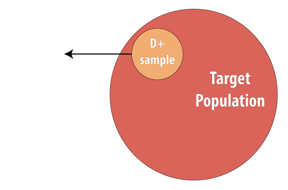
Case-Control
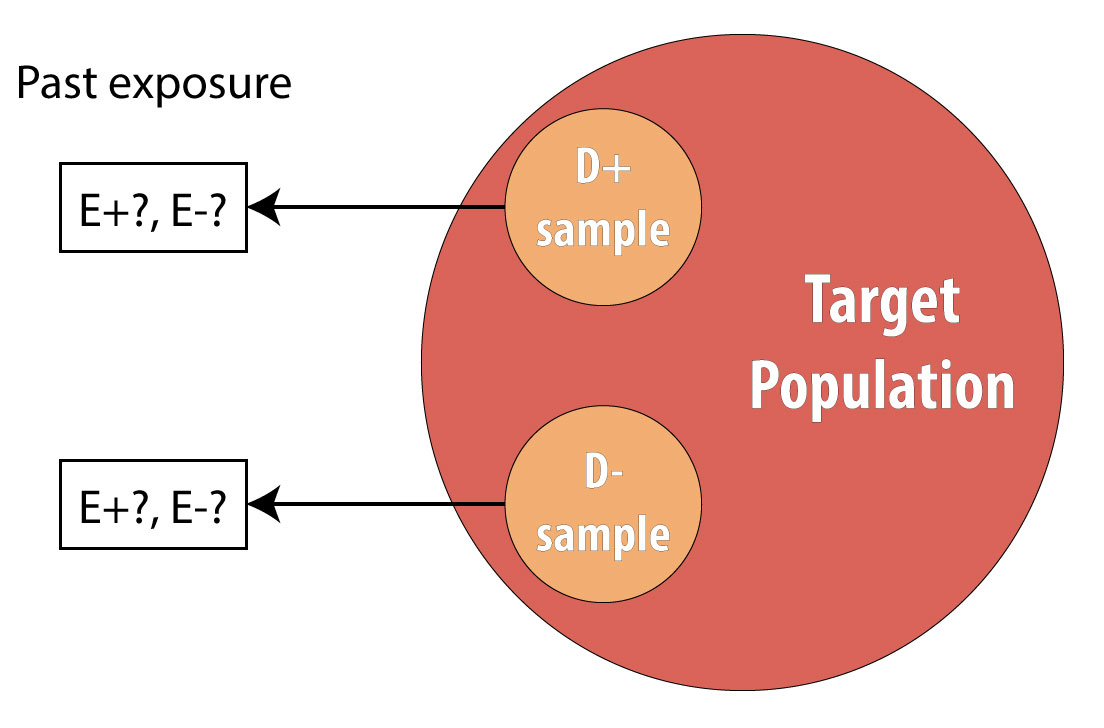
The final type of epidemiologic study that is commonly used is the case-control study. It also begins with prevalent cases and thus is faster and cheaper than longitudinal (prospective cohort or RCT) designs. To conduct a case-control study, one first draws a sample of diseased individuals (cases):
Then a sample of nondiseased individuals (controls):
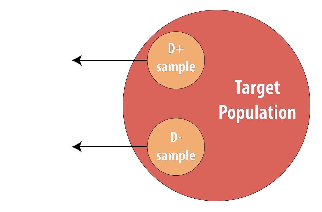
First and foremost, note that both cases and controls come from the same underlying population. This is extremely important, lest a researcher conduct a biased case-control study (see chapter 9 for more on this). After sampling cases and controls, one measures exposures at some point in the past. This might be yesterday (for a foodborne illness) or decades ago (for osteoporosis):
Again, we cannot calculate incidence because we are using prevalent cases, so instead we calculate the OR in the same manner as above. The interpretation is identical, but now we must refer to the time period because we explicitly looked at past exposure data:
Note, however, that one cannot calculate the overall sample prevalence using a 2 × 2 table from a case-control study, because we artificially set the prevalence in our sample (usually at 50%) by deliberately choosing individuals who were diseased for our cases.
Exposure OR versus Disease OR
Technically, for a case-control study, one calculates the disease OR rather than the exposure OR (which is presented under cross-sectional studies). In other words, since in case-control studies we begin with disease, we are calculating the odds of being exposed among those who are diseased compared to the odds of being exposed among those who are not diseased:
\[\mathrm{OR}_{\text {disease }}=\frac{(A / C)}{(B / D)}=\frac{A D}{B C}\]
The exposure odds ratio, you will remember, calculates the odds of being diseased among those who are exposed, compared to the odds of being diseased among those who are unexposed:
\[\mathrm{OR}_{\text {exposure }}=\frac{(A / B)}{(C / D)}=\frac{A D}{B C}\]
In advanced epidemiology classes, one is expected to appreciate the nuances of this difference and to articulate the rationale behind it. However, since both the exposure and the disease odds ratios simplify to the same final equation, here we will not differentiate between them. The interpretation is the same: an OR > 1 means that disease is more common in the exposed group (or exposure is more common in the diseased group—same thing), and an OR < 1 means that disease is less common in the exposed group (or exposure is less common in the diseased group—again, same thing).
Risk Difference
RR and OR are known as relative or ratio measures of association for obvious reasons. These measures can be misleading, however, if the absolute risks (incidences) are small.[2] For example, if a cohort study was done, and investigators observed an incidence in the exposed of 1 per 1,000,000 in 20 years and an incidence in the unexposed, and an incidence in the unexposed of 2 per 1,000,000 in 20 years, the RR would be 0.5: there is a 50% reduction in disease in the exposed group. Break out the public health intervention! However, this ratio measure masks an important truth: the absolute difference in risk is quite small: 1 in a million.
To address this issue, epidemiologists sometimes calculate instead the risk difference instead:
\[RD = I_{E+} – I_{E-}\]
Unfortunately, this absolute measure of association is not often seen in the literature, perhaps because interpretation implies causation more explicitly or because it is more difficult to control for confounding variables (see chapter 7) when calculating difference measures.
Regardless, in our smoking/HTN example, the RD is:
\[\mathrm{RD}=\mathrm{I}_{\mathrm{E}+}-\mathrm{I}_{\mathrm{E}-}=75 \text { per } 100 \text { in } 10 \text { years }-33 \text { per } 100 \text { in } 10 \text { years }=42 \text { per } 100 \text { in } 10 \text { years }\]
Note that the RD has the same units as incidence, since units do not cancel when subtracting. The interpretation is as follows:
Over 10 years, the excess number of cases of HTN attributable to smoking is 42; the remaining 33 would have occurred anyway.
You can see how this interpretation assigns a more explicitly causal role to the exposure.
More common (but still not nearly as common as the ratio measures) are a pair of measures derived from the RD: the attributable risk (AR) and the number needed to treat/number needed to harm (NNT/NNH).
The AR is calculated as RD/IE+. Here,
\[\mathrm{AR}=42 \text { per } 100 \text { in } 10 \text { years } / 75 \text { per } 100 \text { in } 10 \text { years }=56 \%\]
Interpretation:
56% of cases can be attributed to smoking, and the rest would have happened anyway.
Again this implies causality; furthermore, because diseases all have more than one cause (see chapter 10), the ARs for each possible cause will sum to well over 100%, making this measure less useful.
Finally, calculating NNT/NNH (both of which are similar, with the former being for preventive exposures and the latter for harmful ones) is simple:
\[\text{NNT} = \dfrac{1}{\text{RD}\]
In our example,
\[\mathrm{NNH}=1 / 42 \text { per } 100 \text { per } 10 \text { years }=1 / 0.42 \text { per } 10 \text { years }=2.4\]
Interpretation:
Over 10 years, for every 2.4 smokers, 1 will develop hypertension.
For a protective exposure, the NNT (commonly used in clinical circles) is interpreted as the number you need to treat in order to prevent one case of a bad outcome. For harmful exposures, as in our smoking/HTN example, it is the number needed to be exposed to cause one bad outcome. For many drugs in common use, the NNTs are in the hundreds or even thousands.[iii][iv]
Conclusions
Epidemiologic data are often summarized in 2 × 2 tables. There are 2 main measures of association commonly used in epidemiology: the risk ratio/rate ratio (relative risk) and the odds ratio. The former is calculated for study designs that collect data on incidence: cohorts and RCTs. The latter is calculated for study designs that use prevalent cases: cross-sectional studies and case-control studies. Absolute measures of association (e.g., risk difference) are not seen as often in epidemiologic literature, but it is nonetheless always important to keep the absolute risks (incidences) in mind when interpreting results.
Below is a table summarizing the concepts from this chapter:
| Study Design | Methods Summary | Incident or Prevalent Cases? | Preferred Measure of Association |
|---|---|---|---|
| Cohort | Start with a nondiseased sample, determine exposure, follow over time. | Incident | Risk ratio or rate ratio |
| RCT | Start with a nondiseased sample, assign exposure, follow over time | Incident | Risk ration or rate ratio |
| Case-Control | Start with diseased (cases), recruit comparable nondiseased (controls), look at previous exposures | Prevalent | Odds ratio |
| Cross-sectional | From a sample, assess both exposure status and disease status simultaneously | Prevalent | Odds ratio |
References
i. Bodner K, Bodner-Adler B, Wierrani F, Mayerhofer K, Fousek C, Niedermayr A, Grünberger. Effects of water birth on maternal and neonatal outcomes. Wien Klin Wochenschr. 2002;114(10-11):391-395. (↵ Return)
ii. Declercq E. The absolute power of relative risk in debates on repeat cesareans and home birth in the United States. J Clin Ethics. 2013;24(3):215-224.
iii. Mørch LS, Skovlund CW, Hannaford PC, Iversen L, Fielding S, Lidegaard Ø. Contemporary hormonal contraception and the risk of breast cancer. N Engl J Med. 2017;377(23):2228-2239. doi:10.1056/NEJMoa1700732 (↵ Return)
iv. Brisson M, Van de Velde N, De Wals P, Boily M-C. Estimating the number needed to vaccinate to prevent diseases and death related to human papillomavirus infection. CMAJ Can Med Assoc J. 2007;177(5):464-468. doi:10.1503/cmaj.061709 (↵ Return)
- These 4 study designs are the basis for nearly all others (e.g., case-crossover studies are a subtype of case-control studies). A few additional designs are covered in chapter 9, but a firm understanding of the 4 designs covered in this chapter will set beginning epidemiology students up to be able to critically read essentially all of the literature. ↵
- Declercq E. The absolute power of relative risk in debates on repeat cesareans and home birth in the United States. J Clin Ethics. 2013;24(3):215-224 ↵