
1.9: Study Designs Revisited
- Page ID
- 38522

\( \newcommand{\vecs}[1]{\overset { \scriptstyle \rightharpoonup} {\mathbf{#1}} } \)
\( \newcommand{\vecd}[1]{\overset{-\!-\!\rightharpoonup}{\vphantom{a}\smash {#1}}} \)
\( \newcommand{\dsum}{\displaystyle\sum\limits} \)
\( \newcommand{\dint}{\displaystyle\int\limits} \)
\( \newcommand{\dlim}{\displaystyle\lim\limits} \)
\( \newcommand{\id}{\mathrm{id}}\) \( \newcommand{\Span}{\mathrm{span}}\)
( \newcommand{\kernel}{\mathrm{null}\,}\) \( \newcommand{\range}{\mathrm{range}\,}\)
\( \newcommand{\RealPart}{\mathrm{Re}}\) \( \newcommand{\ImaginaryPart}{\mathrm{Im}}\)
\( \newcommand{\Argument}{\mathrm{Arg}}\) \( \newcommand{\norm}[1]{\| #1 \|}\)
\( \newcommand{\inner}[2]{\langle #1, #2 \rangle}\)
\( \newcommand{\Span}{\mathrm{span}}\)
\( \newcommand{\id}{\mathrm{id}}\)
\( \newcommand{\Span}{\mathrm{span}}\)
\( \newcommand{\kernel}{\mathrm{null}\,}\)
\( \newcommand{\range}{\mathrm{range}\,}\)
\( \newcommand{\RealPart}{\mathrm{Re}}\)
\( \newcommand{\ImaginaryPart}{\mathrm{Im}}\)
\( \newcommand{\Argument}{\mathrm{Arg}}\)
\( \newcommand{\norm}[1]{\| #1 \|}\)
\( \newcommand{\inner}[2]{\langle #1, #2 \rangle}\)
\( \newcommand{\Span}{\mathrm{span}}\) \( \newcommand{\AA}{\unicode[.8,0]{x212B}}\)
\( \newcommand{\vectorA}[1]{\vec{#1}} % arrow\)
\( \newcommand{\vectorAt}[1]{\vec{\text{#1}}} % arrow\)
\( \newcommand{\vectorB}[1]{\overset { \scriptstyle \rightharpoonup} {\mathbf{#1}} } \)
\( \newcommand{\vectorC}[1]{\textbf{#1}} \)
\( \newcommand{\vectorD}[1]{\overrightarrow{#1}} \)
\( \newcommand{\vectorDt}[1]{\overrightarrow{\text{#1}}} \)
\( \newcommand{\vectE}[1]{\overset{-\!-\!\rightharpoonup}{\vphantom{a}\smash{\mathbf {#1}}}} \)
\( \newcommand{\vecs}[1]{\overset { \scriptstyle \rightharpoonup} {\mathbf{#1}} } \)
\(\newcommand{\longvect}{\overrightarrow}\)
\( \newcommand{\vecd}[1]{\overset{-\!-\!\rightharpoonup}{\vphantom{a}\smash {#1}}} \)
\(\newcommand{\avec}{\mathbf a}\) \(\newcommand{\bvec}{\mathbf b}\) \(\newcommand{\cvec}{\mathbf c}\) \(\newcommand{\dvec}{\mathbf d}\) \(\newcommand{\dtil}{\widetilde{\mathbf d}}\) \(\newcommand{\evec}{\mathbf e}\) \(\newcommand{\fvec}{\mathbf f}\) \(\newcommand{\nvec}{\mathbf n}\) \(\newcommand{\pvec}{\mathbf p}\) \(\newcommand{\qvec}{\mathbf q}\) \(\newcommand{\svec}{\mathbf s}\) \(\newcommand{\tvec}{\mathbf t}\) \(\newcommand{\uvec}{\mathbf u}\) \(\newcommand{\vvec}{\mathbf v}\) \(\newcommand{\wvec}{\mathbf w}\) \(\newcommand{\xvec}{\mathbf x}\) \(\newcommand{\yvec}{\mathbf y}\) \(\newcommand{\zvec}{\mathbf z}\) \(\newcommand{\rvec}{\mathbf r}\) \(\newcommand{\mvec}{\mathbf m}\) \(\newcommand{\zerovec}{\mathbf 0}\) \(\newcommand{\onevec}{\mathbf 1}\) \(\newcommand{\real}{\mathbb R}\) \(\newcommand{\twovec}[2]{\left[\begin{array}{r}#1 \\ #2 \end{array}\right]}\) \(\newcommand{\ctwovec}[2]{\left[\begin{array}{c}#1 \\ #2 \end{array}\right]}\) \(\newcommand{\threevec}[3]{\left[\begin{array}{r}#1 \\ #2 \\ #3 \end{array}\right]}\) \(\newcommand{\cthreevec}[3]{\left[\begin{array}{c}#1 \\ #2 \\ #3 \end{array}\right]}\) \(\newcommand{\fourvec}[4]{\left[\begin{array}{r}#1 \\ #2 \\ #3 \\ #4 \end{array}\right]}\) \(\newcommand{\cfourvec}[4]{\left[\begin{array}{c}#1 \\ #2 \\ #3 \\ #4 \end{array}\right]}\) \(\newcommand{\fivevec}[5]{\left[\begin{array}{r}#1 \\ #2 \\ #3 \\ #4 \\ #5 \\ \end{array}\right]}\) \(\newcommand{\cfivevec}[5]{\left[\begin{array}{c}#1 \\ #2 \\ #3 \\ #4 \\ #5 \\ \end{array}\right]}\) \(\newcommand{\mattwo}[4]{\left[\begin{array}{rr}#1 \amp #2 \\ #3 \amp #4 \\ \end{array}\right]}\) \(\newcommand{\laspan}[1]{\text{Span}\{#1\}}\) \(\newcommand{\bcal}{\cal B}\) \(\newcommand{\ccal}{\cal C}\) \(\newcommand{\scal}{\cal S}\) \(\newcommand{\wcal}{\cal W}\) \(\newcommand{\ecal}{\cal E}\) \(\newcommand{\coords}[2]{\left\{#1\right\}_{#2}}\) \(\newcommand{\gray}[1]{\color{gray}{#1}}\) \(\newcommand{\lgray}[1]{\color{lightgray}{#1}}\) \(\newcommand{\rank}{\operatorname{rank}}\) \(\newcommand{\row}{\text{Row}}\) \(\newcommand{\col}{\text{Col}}\) \(\renewcommand{\row}{\text{Row}}\) \(\newcommand{\nul}{\text{Nul}}\) \(\newcommand{\var}{\text{Var}}\) \(\newcommand{\corr}{\text{corr}}\) \(\newcommand{\len}[1]{\left|#1\right|}\) \(\newcommand{\bbar}{\overline{\bvec}}\) \(\newcommand{\bhat}{\widehat{\bvec}}\) \(\newcommand{\bperp}{\bvec^\perp}\) \(\newcommand{\xhat}{\widehat{\xvec}}\) \(\newcommand{\vhat}{\widehat{\vvec}}\) \(\newcommand{\uhat}{\widehat{\uvec}}\) \(\newcommand{\what}{\widehat{\wvec}}\) \(\newcommand{\Sighat}{\widehat{\Sigma}}\) \(\newcommand{\lt}{<}\) \(\newcommand{\gt}{>}\) \(\newcommand{\amp}{&}\) \(\definecolor{fillinmathshade}{gray}{0.9}\)Learning Objectives
After reading this chapter, you will be able to do the following:
- Compare and contrast the strengths and limitations of cohort, case-control, cross-sectional, and randomized controlled trial studies
- Describe ecologic studies and explain the ecologic fallacy
- Describe the appropriate use of a systematic review and meta-analysis
Now that we have a firm understanding of potential threats to study validity, in this chapter we will revisit the 4 main epidemiologic study designs, focusing on strengths, weaknesses, and important details. I will also describe a few other study designs you may see, then end with a section on systematic reviews and meta-analyses, which are formal methods for synthesizing a body of literature on a given exposure/disease topic.
Cohorts
Recall from chapter 4 that a cohort study consists of drawing an at-risk (nondiseased) sample from the population, assessing levels of exposure, and then following the cohort over time and watching for incident disease:
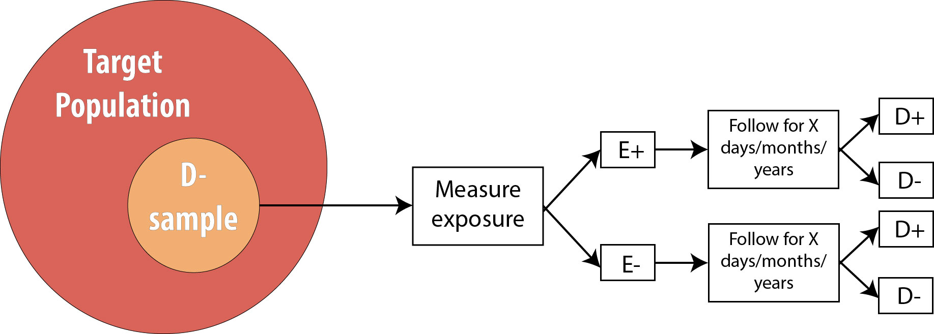
Cohort studies are a very strong study design, meaning that they are less prone to bias and temporality-related logical errors than some other designs. First, because we begin with a non-diseased sample, for which we immediately assess exposure status, we know that the exposure came first. Because of this, cohorts are unlikely to have misclassification of exposure differentially by disease status because the exposure is measured before disease status is known (misclassification of disease status differentially by exposure, however, is still a risk).
Cohort Temporality and Latent Periods
For diseases that have a long latent period—meaning that the biological onset of disease occurs long before the disease is detected and diagnosed—it is possible that some of our “nondiseased” sample are actually diseased but just have not been diagnosed yet. This could happen, for instance, for a cancer patient while their tumor is still too small to detect. When conducting studies on conditions with known or suspected long latent periods, epidemiologists will often exclude from the sample any participants in whom the disease is diagnosed during the first several months of follow-up, theorizing that those individuals were not truly disease-free at baseline.
Second, because cohort studies look for incident disease, they do not conflate the person’s having the disease with how long they have had it, as prevalence studies do (see chapter 2 for a discussion of the mathematical relationship among incidence, prevalence, and duration of disease).
Third, they are the only study design that can be used to assess rare exposures. If the exposure is uncommon within the target population (say, 10% or fewer people can be expected to be exposed), then cohort studies can deliberately sample exposed individuals to ensure sufficient statistical power (the smallest cell in the 2 × 2 table drives the power) without needing an unreasonably large sample. For example, if we are concerned about chemical exposures in a particular factory, we might enroll exposed workers from that factory as well as a unexposed group of workers from a different factory (checking first, of course, to make sure that the second factory is truly exposure-free) and follow both groups, looking for incident disease.
Which leads nicely to the fourth strength: multiple outcomes can be assessed in the same cohort. In our factory example above, the exposed workers from Factory 1 and the unexposed workers from Factory 2 can be followed for any reasonably common disease. (Just how common is a judgment call—we could also watch for and track uncommon diseases, as long as we acknowledge that those analyses would be underpowered.) We could look for new-onset heart disease, leukemia, fibromyalgia, diabetes, death, or anything else of interest. If looking at more than one outcome, then we also must measure all outcomes of interest in the sample at baseline. Then, for analyses of each specific outcome, we merely eliminate from the cohort the people who were not at risk of that outcome. For instance, if Person A joins our factory study, and at the beginning of the study they already have hypertension but do not have melanoma, then we would not include that person in analyses where hypertension is the disease outcome. Their data could, however, be included in analyses where melanoma is the disease outcome, because they were at risk of melanoma at baseline.
Cohort studies can also be used to study multiple exposures, as long as these exposures are all common enough that we would not need to deliberately sample on exposure status. To do this, we would just grab a sample from the target population, and assess a multitude of exposures. If we want to also assess more than one outcome, then we need to measure all disease states of interest at baseline so that eventual analyses can be restricted to the population at risk, as discussed above. This ability to look at multiple outcomes—and potentially also multiple exposures—adds efficiency to cohort studies, as we can essentially conduct numerous studies all at once.
The Framingham Heart Study is a classic example of a cohort study that assessed multiple exposures and multiple outcomes. This study, a collaboration between the US National Heart, Lung, and Blood Institute (a division of the National Institutes of Health) and Boston University, began in 1948 by enrolling just over 5,000 adults living in Framingham, Massachusetts. Investigators measured numerous exposures and outcomes, then repeated the measurements every few years. As the cohort aged, their spouses, children, children’s spouses, and grandchildren have been enrolled. The Framingham study is responsible for much of our knowledge about heart disease, stroke, and related disorders, as well as of the intergenerational effects of some lifestyle habits. More information and a list of additional publications (more than 3,500 studies have been published using Framingham data) can be found here.
Cohort studies also have downsides. They cannot be used to study rare diseases because the cohort would need to be too large to be practical. For example, phenylketonuria is a genetic metabolic disorder affecting about 1 in 10,000 infants born in the US.1 To get even 100 affected individuals, then, we would need to enroll one million pregnant women in our study—a number that is neither practical nor feasible.
Furthermore, prospective cohort studies are costly. Following people over time takes a fair bit of effort, which means that study personnel costs are high. Because of this, cohort studies cannot be used to study diseases with decades-long induction or latent periods.
For example, it would be difficult to conduct a cohort study looking at whether adolescent dairy product consumption is associated with osteoporosis in 80-year-old women, because following current teenagers for 60 years or more would be extremely difficult. Along similar lines, selection biases related to lack of follow-up can be severe in studies with long durations: the longer we try to follow people, the more likely it is that they move, change phone numbers/email addresses, or get tired of filling out a survey every year and just stop participating. More troubling would be if people who start to feel ill are the ones who quit answering inquiries from the study team. What if these people were feeling ill because they were about to be diagnosed with the outcome under study? Despite this difficulty, a few long cohort studies such as Framingham exist and have yielded rich datasets and much knowledge about human health.
Randomized Controlled Trials
Recall from chapter 4 that an RCT is conceptually just like a cohort, with one difference: the investigator determines exposure status.
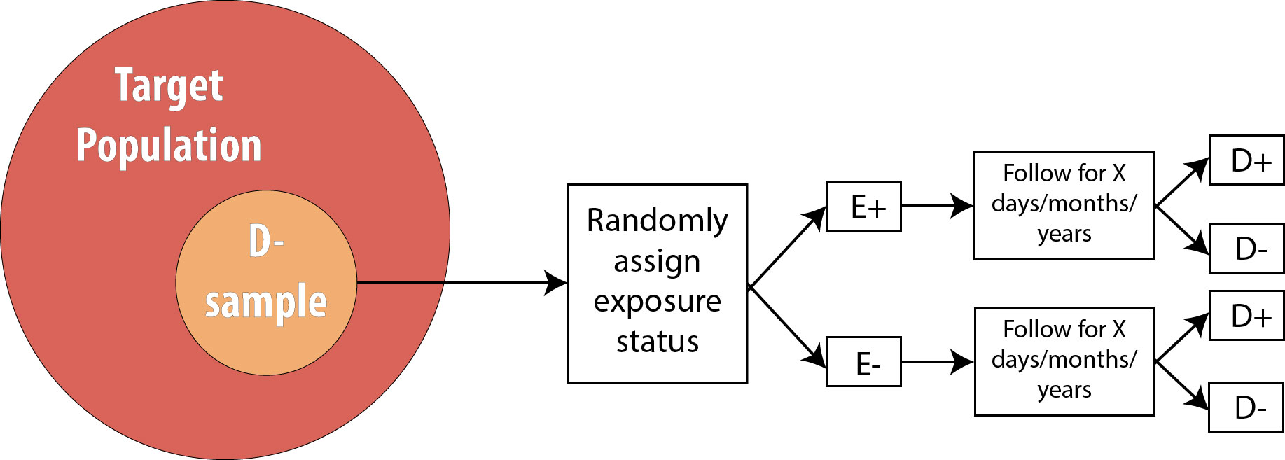
Thus all of the strengths and weaknesses of cohort studies apply also to RCTs, with one exception: to study multiple exposures, one would need to re-randomize for each exposure. A few studies have successfully done this (the Women’s Health Initiative, for instance, randomized women to both hormone replacement therapy or placebo, and also, separately, to calcium supplements or placebo), but practically speaking RCTs are usually limited to one exposure.
One additional strength of a randomized trial (which does not apply to cohort studies) is that if the study is large enough (at least several hundred participants) and exposure allocation is truly random (i.e., not “every other person” or some other predictable scheme), then there will be no confounding. One can control, statistically, for measured confounders in a cohort study (see chapter 7), but what about any unknown and/or unmeasured confounders? The key feature of randomization is that it accounts for all confounders: known, unknown, measured, and unmeasured.
Recall from chapter 7 that for a variable to act as a confounder, it must satisfy these conditions:
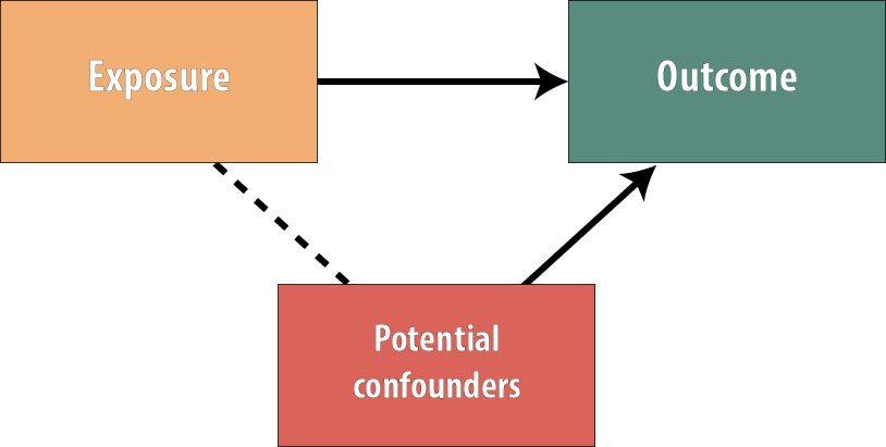
The variable must cause the outcome, be statistically associated with the exposure, and not be on the causal pathway (so the exposure does not cause the confounder). By randomly assigning the exposure, we have ensured that no variables exist that are associated with the exposure.
The picture now looks like this:
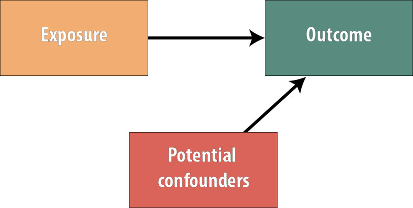
Because no variables are more common in the exposed group than the unexposed group (or vice versa), we have gotten rid of all possible confounding. The benefits of this in terms of internal study validity cannot be overstated.
However, RCTs also have limitations, and these should not be overlooked. First and foremost, they are even more expensive than cohort studies. Second, there are often ethical considerations rendering the randomized trial design unusable. For instance, at this point, we could not ethically justify randomizing people to a smoking exposure (because its harms are so well-documented, we cannot ask people to begin smoking for our study). We also cannot randomize where people live, but certainly where people live has a profound effect on their health.ii Observational studies of these exposures, on the other hand, are ethically viable because people have already chosen whether to smoke and where to live, and the epidemiologist merely measures these existing exposures.
Third, RCTs often have generalizability issues because the kinds of people who are willing to participate in a study where they (the participant) do not get to choose which study group to be in are not a random subset of the overall population. For instance, if the only people who have time to participate in our physical activity intervention are people who are retired, then can we generalize to the (presumably younger) population who are still working? Perhaps—but perhaps not. Investigators conducting RCTs also sometimes overly restrict the inclusion criteria to the extent that results are not generalizable to the overall population. For instance, a well-known trial of blood pressure control in older adults excluded those with diabetes, cancer, and a host of other comorbidities.iii Given that most older people have at least one of these chronic diseases, to whom can we really apply the results?
Lastly, we have to precisely specify the exposure in an RCT. If we are doing a physical activity intervention, are we going to ask those randomized to the exposed group to walk? To take a yoga class? Do supervised strength training? If so, how much? How often? With how much intensity? For how many weeks or months? In a cohort study, we would assess the physical activity people are doing anyway, and there would be a huge variety of responses, which we could then categorize in any number of ways. With a randomized trial, we have to decide on all of the details. If we are wrong, or if we apply the intervention at the wrong time in the disease process, it could seem like there is no exposure/disease association, when really there is and our exposure was slightly off somehow.
Randomized trials are often called the “gold standard” of epidemiologic and clinical research because of their ability to minimize confounding. However, their drawbacks are substantial, and well-conducted observational studies should not necessarily be discounted merely because they are not RCTs. Nonetheless, RCTs play an enormous role particularly in medicine, as the Food and Drug Administration (FDA) requires multiple RCTs prior to approving new drugs and medical devices. Because of the FDA’s strict requirements, protocols for randomized trials must be registered (at clinicaltrials.gov) prior to the start of any data collection.
Outside of pharmaceutical research and development, RCTs, because of their methodologic strengths, have the potential to change practice when evidence from new, large, well-designed studies emerge. For example, in 2005 Dr. Paul Ridker and colleagues absolutely changed the way physicians thought about heart disease prophylaxis in women.iv Prior to publication of this large (20,000 women in each group) trial, we assumed that, like men, older women should take a baby aspirin every other day to prevent heart attacks. However, the Ridker trial showed that aspirin acts differently in women (gender is an effect modifier!), and the aspirin-a-day-prevents-heart-attacks regimen will not work for most women.
Case-Control Studies
A case-control study is a retrospective design wherein we begin by finding a group of cases (people who have the disease under study) and a comparable group of controls (people who do not have the disease):
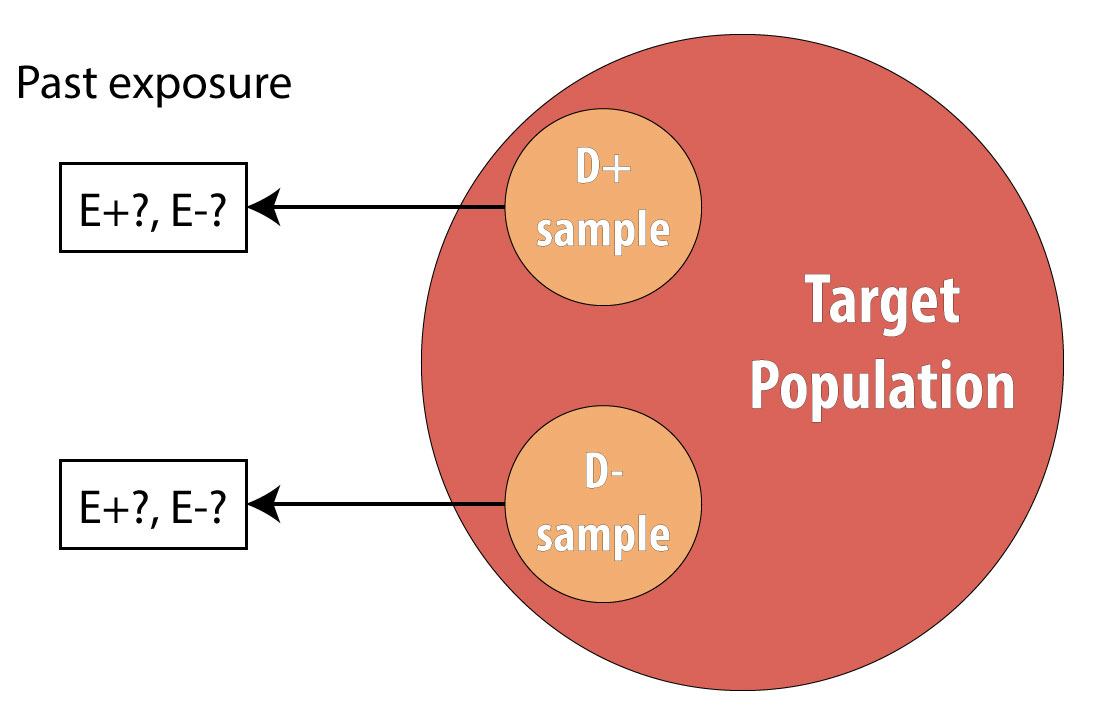
A common mistake made by beginning epidemiology students is to state that “cases are people with the disease, who are exposed.” This is incorrect. Cases are people with the disease, and to avoid differential misclassification, it is important that both cases and controls be recruited without regard for exposure status. Once we have identified all cases and controls, then we assess which people were exposed.
Because they do not require following people over time, case-control studies are much cheaper to conduct than cohorts or randomized trials. They also provide an efficient way to study rare diseases and diseases with long induction and/or latent periods. Case-control studies can assess multiple exposures, though they are limited to one outcome by definition.
Case-control studies assess exposure in the past. Occasionally, these past exposure data come from existing records (e.g., medical records for a person’s blood pressure history), but usually we rely on questionnaires. Case-control studies are thus subject to recall bias, more so than prospective designs. Epidemiologists conducting case-control studies need to be particularly wary of differential recall by case status. It is plausible that people with a given condition will have spent time thinking about what might have caused it and thus be able to report past exposures with greater detail than members of the control group. Regardless of case status, the questions asked must be possible for people to answer. No one can say with certainty exactly what they ate on a particular day a decade ago; however, most people can probably recall what kinds of foods they usually ate on most days. Details are thus sacrificed in favor of bigger-picture accuracy (which may still be of questionable validity, depending on people’s memories). Remember from chapters 5 and 6: ask yourself, “Can people tell me this? Will people tell me this?”
The proper selection of controls is paramount in case-control studies, but unfortunately, who constitutes a “proper” control is not always immediately obvious. To avoid selection biases, cases and controls must come from the same target population—that is, if controls had been sick with the disease in question, they too would have been cases.
For instance, if cases are recruited from a particular hospital, then controls should be sampled from the population of people who also would have sought care at that hospital if necessary. This seems simple enough, but it is not always easy to translate into practice. If we are studying traumatic brain injury (TBI) in children in Oregon, a good place to find cases would be at Doernbecher Children’s Hospital in Portland. Other hospitals throughout the Pacific Northwest send kids with severe TBIs to Doernbecher, where a myriad of pediatric specialists are available to care for them; this hospital thus has a sufficient number of cases for our study.
Where would we get controls? One possibility would be to take as controls other children who are patients at Doernbecher, for a condition other than TBI. This satisfies the criterion that controls would also get care at this hospital, because they are getting care at this hospital. However, to the extent that kids receiving care for other conditions might also have unusual exposure histories, this could lead to biased estimates of association. Another option would be to designate as controls children who are not sick, sampled perhaps from a Portland neighborhood or two. However, this would also lead to selection bias, because Doernbecher is a referral hospital, receiving as patients children from a several-hundred-mile radius, not just children who live in Portland. If kids who live out in more rural areas are different than those who live in the city, we would have biased estimates of association.
The bottom line is that there is no perfect way to recruit controls, and epidemiologists love to poke holes in other people’s control groups for case-control studiesv,vi (this is considered good sport at epidemiology conferences). One way to reduce bias from the control group is to recruit multiple control groups—perhaps one hospital-based and one community-based. If the results are not substantially different, then any selection biases that are operating are perhaps not overly influencing the results.
For long-lasting chronic diseases, the issue of disease duration again comes into play. To avoid temporality issues, we must know at a minimum the date of diagnosis and ensure that we are assessing exposures that happened well before that date. For conditions for which the induction and latent periods are unknown, investigators will sometimes conduct a case-control study that recruits incident cases of disease over a period of several months. Thus as soon as cases are recruited, we can ask about past exposures with the confidence that at least the case diagnosis occurred after those exposures. While a long latent period might still be an issue, one way around this would be to ask about exposures over multiple time periods—say, 0–5 years ago, 6–10 years ago, 11–15 years ago, and so on—and compare results across these windows.
Despite these difficulties, case-control studies have made substantial contributions to our knowledge about health over the years. The surgeon general’s 1964 report Smoking and Healthvii, for instance, was based on literature that stemmed from a case-control study conducted by Richard Doll and Austin Bradford Hill.viii
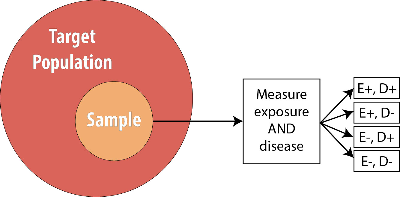
Cross-Sectional Studies
Recall from chapter 4 that in a cross-sectional study, we draw a single sample from the target population and assess current exposure and disease status on everyone:
The main strength of cross-sectional studies is that they are the fastest and cheapest studies to conduct. They are thus used for many surveillance activities—the National Health and Nutrition Examination Survey (NHANES), Pregnancy Risk Assessment Monitoring System (PRAMS), and Behavioral Risk Factor Surveillance System (BRFSS) are all cross-sectional studies that are repeated with a new sample each year (see chapter 3)—and in other situations where resources may be limited and/or immediate answers are required.
Cross-sectional studies are limited by the fact that we sample for neither exposure nor disease and that we instead “get what we get” when drawing our sample from the population. They thus cannot be used for either rare exposures or rare diseases.
Another limitation is that we have no data on temporality: we do not know whether the exposure or the disease came first because we are measuring the prevalence of both at the same point in time.
Cross-sectional studies along with surveillance (which looks only at measures of disease frequency, not at exposure/disease relationships) are thus limited to hypothesis generation activities. We cannot make (nonsurveillance) public health or clinical decisions based on evidence only from these studies.
Case Reports/Case Series
In the clinical literature, one often sees case reports. These are short blurbs reporting an interesting and unusual patient seen by a particular doctor or clinic. A case series is the same thing but describes more than one patient—usually only a few,ix,x but sometimes several hundred.xi Case reports and case series have little value for epidemiologists because they are not studies per se; they have no comparison groups. If a case series is published saying that 45% of patients in this series with disease Y also have disease Z, this is not useful information for an epidemiologist. How many patients who do not have disease Y also have disease Z? Without data on a comparable group of patients who do not have disease Y, there is nothing to be done with the 45% data point given in the case series.
That said, case reports and case series can be extremely useful for public health professionals. Because by definition they present data from unusual patients, they can often act as a kind of sentinel surveillance, drawing our attention to a new, emerging public health threat. For example, in 1941, a physician from Australia noticed an increase in a kind of birth defect affecting infant eyes. He published this as a case series,xii hypothesizing that maternal rubella infection was the cause. Other physicians from around the world chimed in that they, too, had seen a recent sudden increase in this birth defect in women whose pregnancies were complicated by rubella,xiii,xiv,xv leading to our current practice of checking for rubella antibodies in all pregnant women and vaccinating those without immunity. As another example, in the early 1980s, a set of case series published by the Centers for Disease Control and Prevention (CDC) in its Morbidity and Mortality Weekly Report drew our attention to unusual kinds of cancers and opportunistic infections occurring in otherwise young, healthy populations—our first inkling of the HIV/AIDS epidemic.x,xvi,xvii,xviii More recently, in 2003, case reports detailing an unusual, deadly respiratory infection in people traveling to Hong Kong led to increased global public health and clinical awareness of this unusual set of symptoms, allowing immediate quarantine of affected individuals who had traveled back to Toronto.xix,xx,xxi This quick action prevented SARS from becoming a global pandemic.
Ecologic Studies
Ecologic studies are those in which group-level data (usually geographic) are used to compare rates of disease and/or disease behaviors. For instance, this picture showing variation in seat belt use by state from chapter 1 is a kind of ecologic study:
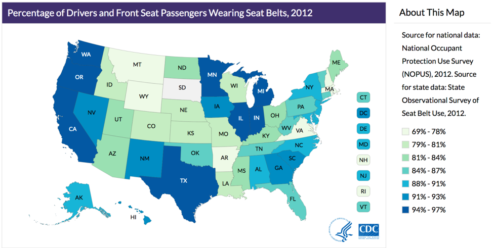
By comparing rates of seat belt use across different states, we are comparing group-level data, not data from individuals. While useful, this kind of picture can lead to many errors in logic. For example, it assumes that everyone in a given state is exactly the same—obviously this is not true. While it is true that on average, people in Oregon wear their seat belt more often than people from Idaho, this does not mean that everyone in Oregon wears their seat belt more often than everyone in Idaho. We could easily find someone in Oregon who never wears their seat belt and someone in Idaho who always does.
The above logical error—ascribing group-level numbers to any one individual—is an example of the ecologic fallacy. This also comes into play when looking at both exposure and disease patterns using group-level data, as in this example, looking at per-capita rice consumption and maternal mortality in each country:
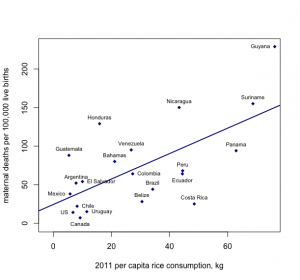
Figure 9-8. Created with data from here and here.
From looking at this graph, it appears that the more rice that is consumed by citizens of a particular country, the higher the maternal mortality rate. The ecologic fallacy here would stem from assuming that it is the rice consumers who are dying from complications related to pregnancy or birth, but we cannot know whether this is true using only group-level data.
With all of these problems, then, why conduct ecologic studies? Even more so than cross-sectional studies, they are quick and cheap. They also always use preexisting data—census estimates for per-county income; the amount of some product (such as rice) consumed by a given group of people (often tracked by sellers of that product); and recorded information on the prevalence of certain diseases (usually publicly available via the websites of health ministries for various countries or as by-country comparisons published by the World Health Organization). The use of ecologic studies is limited only to hypothesis generation, but they are so easy that they can be a good first step for a totally new research question.
Systematic Reviews and Meta-analyses
Because epidemiology relies on humans, it is more prone to both bias and confounding than other sciences. Does this render it useless? Absolutely not, though one must have a robust appreciation for the assumptions and limitations inherent in epidemiologic studies. One of these limitations is that barring exceptionally well-done, randomized controlled trials (as the Ridker trial,iv mentioned previously), we rarely change public health or clinical policy based on just one epidemiologic study. Rather, we do one study, then another, and then another, using better and better study designs until eventually there is a body of evidence on a topic that stems from different populations, uses different study designs, perhaps measures the exposure in slightly different ways, and so on. If all these studies tend to show the same general results (as did all the early studies on smoking and lung cancer), then we start to think that the association might be causal (see chapter 10 for more detail on this) and implement public health or clinical changes.
When results of existing studies on a topic are more mixed, there is a formal way of synthesizing their results across all of them, to arrive at “the” answer: meta-analysis (or systematic review—they differ slightly, as discussed below). The procedure for either of these is the same:
- Determine the topic—precisely. Do we care about correlates of physical activity in kids generally, or only in PE class at school? Only at home? Everywhere? Is our focus all children or only grade-school kids? Only adolescents? There often is no right answer, but as with defining our target population (see chapter 1), this needs to be decided ahead of time.
- Systematically search the literature for relevant papers. By systematically, I mean using and documenting specific search terms and placing documented limits (language, publication date, etc.) on the search results. The key is to make the search replicable by others. It is not acceptable to just include papers that authors are aware of without searching the literature for others—doing so results in a biased sample of all the papers that should have been included.
- Narrow down the search results to only those directly addressing the topic as determined in Step 1.
- For each of the studies to be included, abstract key data: the exposure definition and measurement methods, the outcome definition and measurement methods, how the sample was drawn, the target population, the main results, and so on.
- Determine whether the papers are similar enough for meta-analysis (there are formal statistical procedures to test for this, which are beyond the scope of this book).xxii(p287)
- If they are, then researchers essentially combine all the data from all the included studies and generate an “overall” measure of association and 95% confidence interval.
- If they are not, then the authors will synthesize the studies in other meaningful ways, comparing and contrasting their results, strengths, and weaknesses and arriving at an overall conclusion based on the existing literature. An overall measure of association is not calculated, but usually the authors are able to conclude that some exposure either is or is not associated with some outcome (and perhaps roughly the strength of that association).
- Assess the likelihood of publication bias (again, there are formal statistical methods for this)xxii(pp197-200) and the degree to which that may or may not have affected the results.
- Publish the results!
Ideally, at least 2 different investigators will conduct steps 2–4 completely independently of each other, checking in after completion of each step and resolving any discrepancies, usually by consensus.xxiii This provides a check against un- or subconscious bias on the part of the authors (remember: we’re all human and therefore all biased). For systematic reviews and meta-analyses conducted after 2015 or so, the protocol for the review (search strategy, exact topic, etc.) should be registered prior to step 2 with a central registry, such as PROSPERO. This provides a check against bias—authors who deviate from their preregistered protocols should provide very good reasons for doing so, and such studies should be interpreted with extreme caution.
Results from meta-analyses are often presented as forest plots that plot each included study’s main result (with the size of the square corresponding to sample size) and an overall estimate of association is indicated as a diamond at the bottom. Here is an example from a meta-analysis of chocolate consumption and systolic blood pressure (SBP, the top number in a blood pressure reading):
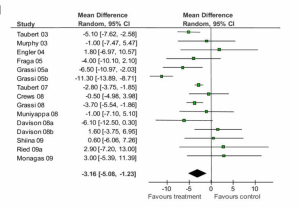
Figure 9-9. Adapted from Reid et.al., BMC Medicine 2010
You can see from this forest plot that the majority of studies showed a decrease in SBP for people who ate more chocolate, though not all studies found this. Some point estimates are quite close to 0.0 (which is the “null” value here, because we’re looking at change in a single number, not a ratio), and 10 of the confidence intervals cross 0.0, indicating that they are not statistically significant. Nonetheless, 6 studies–the largest studies, since their confidence intervals are the narrowest–are statistically significant, and all of these in the direction of chocolate being beneficial. Indeed, the overall (or “pooled”) change in SBP and 95% CI shown at the bottom (the black diamond) indicates a small (approximately 3 mm Hg) reduciton in SBP for chocolate consumers. Does this mean we should all start eating lots of chocolate? Not necessarily: a 3 mm Hg (“millimeters of mercury”–still the units in which we measure blood pressure, despite mercury not being involved for several decades now) drop in SBP is not clinically significant. A normal SBP is between 90 and 120, so a 3 mm Hg drop puts you at 87-117–likely not even a noticeable physiologic change.
As alluded to above, meta-analysis requires a certain similarity among the studies that will be pooled (e.g., they need to control for similar, if not identical, confounders). Often, this is not the case for a given body of literature—in which case, the authors will systematically examine all the evidence and do their best to come up with “an” answer, taking into consideration the quality of individual studies, the overall pattern of results, and so on. For example, in a systematic review of risk-reducing mastectomy (RRM), the prophylactic surgical removal of breasts in women who do not yet have breast cancer, but who have the BRCA-1 or BRCA-2 genes and thus are at very high risk (where BRRM refers to bilateral RRM—having both breasts removed). The authors described the overall results of this study as follows:
Twenty-one BRRM studies looking at the incidence of breast cancer or disease-specific mortality, or both, reported reductions after BRRM, particularly for those women with BRCA1/2 mutations.…Twenty studies assessed psychosocial measures; most reported high levels of satisfaction with the decision to have RRM but greater variation in satisfaction with cosmetic results. Worry over breast cancer was significantly reduced after BRRM when compared both to baseline worry levels and to the groups who opted for surveillance rather than BRRM, but there was diminished satisfaction with body image and sexual feelings.xxvii(p2)
The authors then concluded:
While published observational studies demonstrated that BRRM was effective in reducing both the incidence of, and death from, breast cancer, more rigorous prospective studies are suggested. [Because of risks associated with this surgery] BRRM should be considered only among those at high risk of disease, for example, BRCA1/2 carriers.xxvii(p2)
No overall “pooled” estimate of the protective effect associated with RRM is provided, but the authors are nonetheless able to convey the overall state of the literature, including where the body of literature is lacking.
Systematic reviews and meta-analyses are excellent resources for learning about a topic. Realistically, no one has the time to keep up with the literature in anything other than a very narrow topic area, and even then it is really only a boon to researchers in that field to take note of new individual studies. For public health professionals and clinicians not routinely engaging in research, relying on systematic reviews and meta-analyses provides a much better overall picture that is potentially less prone to the biases found in individual studies. However, care must be taken to read well-done reviews. The title of the paper should include either systematic review or meta-analysis, and the methods should mirror those outlined above. Be wary of review papers that are not explicitly systematic—they are extremely prone to biases on the part of the authors and probably should be ignored.[1]
Conclusions
The figure below is a representation of the relative cost and internal validity of the study designs discussed in this chapter:
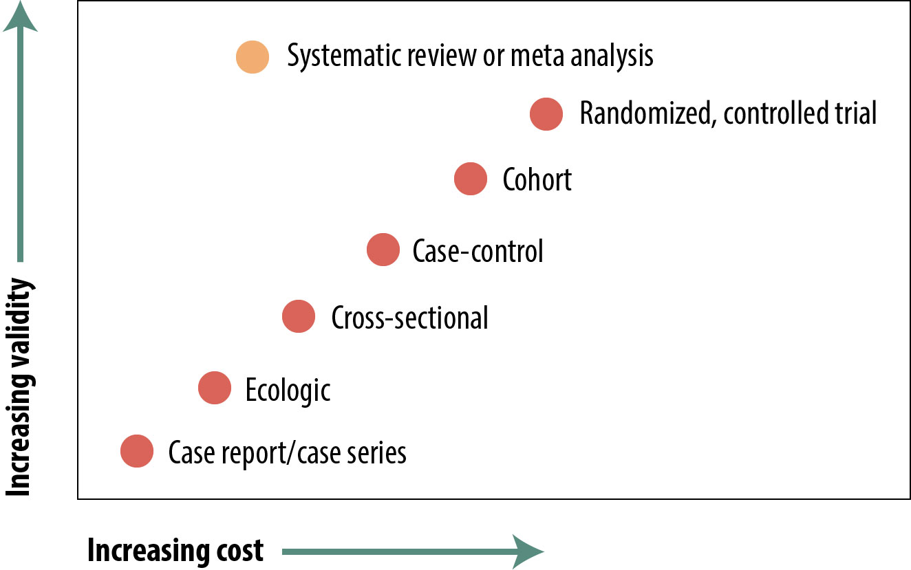
There are many types of epidemiologic studies, from reports of a single, unusual patient up to formal meta-analyses of dozens of other studies. The relative validity of these in terms of using their evidence to shape policy varies widely, but with the exception of review papers, the “better” studies are the more expensive and time-consuming ones. Review papers in and of themselves are not particularly expensive, but they cannot be done until numerous other studies have been published, so if you include those as indirect costs, they take a lot of time and money. The 4 main study types (cross-sectional, case-control, cohort, and RCT) each have strengths and weaknesses, and readers of the epidemiologic literature should be aware of these. There are occasions, independent of cost or validity considerations, when one design or another is preferred (e.g., case-control for rare diseases).
References
i. Williams RA, Mamotte CD, Burnett JR. Phenylketonuria: an inborn error of phenylalanine metabolism. Clin Biochem Rev. 2008;29(1):31-41.
ii. Could where you live influence how long you live? RWJF. https://www.rwjf.org/en/library/inte...ngyoulive.html. Accessed February 19, 2019.
iii. A randomized trial of intensive versus standard blood-pressure control. N Engl J Med. 2017;377(25):2506. doi:10.1056/NEJMx170008
iv. Ridker PM, Cook NR, Lee I-M, et al. A randomized trial of low-dose aspirin in the primary prevention of cardiovascular disease in women. N Engl J Med. 2005;352(13):1293-1304. doi:10.1056/NEJMoa050613. (↵ Return 1) (↵ Return 2)
v. Wacholder S, McLaughlin JK, Silverman DT, Mandel JS. Selection of controls in case-control studies, I: principles. Am J Epidemiol. 1992;135(9):1019-1028. (↵ Return)
vi. Wacholder S, Silverman DT, McLaughlin JK, Mandel JS. Selection of controls in case-control studies, II: types of controls. Am J Epidemiol. 1992;135(9):1029-1041. (↵ Return)
vii. Health CO on S and. Smoking and tobacco use: history of the Surgeon General’s Report. Centers for Disease Control and Prevention. 2017. http://www.cdc.gov/tobacco/data_stat...s/sgr/history/. Accessed October 30, 2018. (↵ Return)
viii. Doll R, Hill AB. Smoking and carcinoma of the lung. Br Med J. 1950;2(4682):739-748. (↵ Return)
ix. Bowden K, Kessler D, Pinette M, Wilson E. Underwater birth: missing the evidence or missing the point? Pediatrics. 2003;112(4):972-973.
x. Centers for Disease Control and Prevention (CDC). A cluster of Kaposi’s sarcoma and Pneumocystis carinii pneumonia among homosexual male residents of Los Angeles and Orange counties, California. MMWR Morb Mortal Wkly Rep. 1982;31(23):305-307.
xi. Cheyney M, Bovbjerg M, Everson C, Gordon W, Hannibal D, Vedam S. Outcomes of care for 16,924 planned home births in the United States: the Midwives Alliance of North America statistics project, 2004 to 2009. J Midwifery Womens Health. 2014;59(1):17-27. (↵ Return)
xii. Gregg NM. Congenital cataract following German measles in the mother. Trans Opthalmol Soc Aust. 1941;3:35-46. (↵ Return)
xiii. Greenberg M, Pellitteri O, Barton J. Frequency of defects in infants whose mothers had rubella during pregnancy. J Am Med Assoc. 1957;165(6):675-678. (↵ Return)
xiv. Manson M, Logan W, Loy R. Rubella and Other Virus Infections during Pregnancy. London: Her Royal Majesty’s Stationery Office; 1960. (↵ Return)
xv. Lundstrom R. Rubella during pregnancy: a follow-up study of children born after an epidemic of rubella in Sweden, 1951, with additional investigations on prophylaxis and treatment of maternal rubella. Acta Paediatr Suppl. 1962;133:1-110. (↵ Return)
xvi. Centers for Disease Control (CDC). Possible transfusion-associated acquired immune deficiency syndrome (AIDS)—California. MMWR Morb Mortal Wkly Rep. 1982;31(48):652-654. (↵ Return)
xvii. Centers for Disease Control (CDC). Pneumocystis pneumonia—Los Angeles. MMWR Morb Mortal Wkly Rep. 1981;30(21):250-252. (↵ Return)
xviii. Centers for Disease Control (CDC). Unexplained immunodeficiency and opportunistic infections in infants—New York, New Jersey, California. MMWR Morb Mortal Wkly Rep. 1982;31(49):665-667. (↵ Return)
xix. Centers for Disease Control and Prevention (CDC). Severe acute respiratory syndrome—Singapore, 2003. MMWR Morb Mortal Wkly Rep. 2003;52(18):405-411. (↵ Return)
xx. Centers for Disease Control and Prevention (CDC). Update: severe acute respiratory syndrome—United States, May 14, 2003. MMWR Morb Mortal Wkly Rep. 2003;52(19):436-438. (↵ Return)
xxi. Centers for Disease Control and Prevention (CDC). Cluster of severe acute respiratory syndrome cases among protected health-care workers—Toronto, Canada, April 2003. MMWR Morb Mortal Wkly Rep. 2003;52(19):433-436. (↵ Return)
xxii. Egger M, Smith GD, Altman DG, eds. Systematic Reviews in Health Care: Meta-analysis in Context. London: BMJ Publishing; 2001. (↵ Return 1) (↵ Return 2)
xxiii. Harris JD, Quatman CE, Manring MM, Siston RA, Flanigan DC. How to write a systematic review. Am J Sports Med. 2014;42(11):2761-2768. doi:10.1177/0363546513497567 (↵ Return)
xxiv. Gilbert R, Salanti G, Harden M, See S. Infant sleeping position and the sudden infant death syndrome: systematic review of observational studies and historical review of recommendations from 1940 to 2002. Int J Epidemiol. 2005;34(4):874-887. doi:10.1093/ije/dyi088
xxv. CDC. Safe sleep for babies. Centers for Disease Control and Prevention. 2018. https://www.cdc.gov/vitalsigns/safesleep/index.html. Accessed January 10, 2019
xxvi. Task Force on Sudden Infant Death Syndrome, Moon RY. SIDS and other sleep-related infant deaths: expansion of recommendations for a safe infant sleeping environment. Pediatrics . 2011;128(5):1030-1039.
xxvii. Carbine NE, Lostumbo L, Wallace J, Ko H. Risk-reducing mastectomy for the prevention of primary breast cancer. Cochrane Database Syst Rev. 2018;4:CD002748. doi:10.1002/14651858.CD002748.pub4 (↵ Return 1) (↵ Return 2)
- Metasynthesis is a legitimate technique for systematic reviewing qualitative literature. The papers to watch out for are the ones called “integrative review,” “literature review,” or just “review”—anything that is not “systematic review.” ↵