21.8: Analyses when communities have been randomized

In some intervention studies, communities, rather than individuals, are used as the unit of randomization. If this has been done, it is inappropriate to base analyses on responses of individuals, ignoring the fact that randomization was over larger units. An appropriate method of analysis would be to summarize the response in each sampling unit by a single value and analyse these summary values as though they were individual values.

The analysis of such trials, often called ‘cluster randomized trials’, is not straightforward, and only simple methods for performing statistical tests are given here. A comprehensive discussion of the design and analysis of such trials is given in Hayes and Moulton (2009).

8.1 Calculation of standardized responses

Often, trials in which communities have been randomized suffer from problems with confounding variables. If the number of units randomized is large, confounding vari- ables are likely to balance out between groups, but, if the number of units is small (as may be the case when communities have been randomized, even though the number of individuals in each community is large), confounding may be a potentially serious problem, and some adjustment should be made in the analysis. One method of doing this is by standardization.

Within each community, the sampled population is divided into strata on the basis of the confounding variable(s) (for example, age and sex groups). The average value of the outcome measure is computed for those in each stratum (for example, a disease incidence rate). A weighted average of the rates in the different strata is then computed to give a single ‘standardized’ measure for the community, the weights being based on some ‘standard’ population. The same standard population is used for each community, and thus the standardized measures for each community are not biased by the differ- ential composition of each community, with respect to the confounding variable that is being standardized for.

This method is called the ‘direct’ method of standardization. If the number of individ- uals in some strata is small, it may be better to use the ‘indirect’ method, and details of both are given (see Armitage and Berry (1987) for a more detailed discussion of these methods).

Consider a community in which disease risks \(p^i\) have been measured for individ- uals in k strata (for example, age groups). This may be represented in Table 21.17. Also shown are the corresponding data for a ‘standard’ population. For example, this might be chosen as the combined data for all communities in the study.

The directly standardized disease risk for the community (standardized to the stand- ard population) is given by:

\((∑p_iN_i)/∑N_i\)

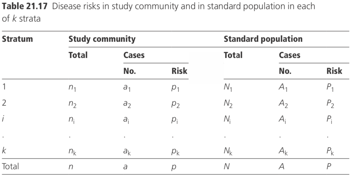
The indirectly standardized disease risk for the community is given by:

\( [∑a_i/(∑n_iP_i)]/(A/N)\)

Having calculated standardized values for each community, the means of the standardized values for the intervention communities may be compared with those for the control communities, using a simple t-test (see Section 6.2).

It is usually safer, however, to perform a non-parametric test if the assumptions underlying the t-test are in any doubt (Armitage and Berry, 1987)), as it may be impossible to verify the assumptions if the study involves a small number of communities.

8.2 Non-parametric rank sum test

Suppose there are n₁ communities in one group and n₂ in the other \(\left( n _ { 1 } \leq n _ { 2 } \right)\) and a summary response has been derived for each community. To perform a non-parametric test, consider all the(n₁ +n₂)observations together, and rank them, giving a rank of 1 to the smallest value and \(\left( n _ { 1 } + n _ { 2 } \right)\) to the highest. Tied ranks are allotted the mid rank of the group. Let T₁ = sum of the ranks in group 1 with n1 observations. Under the null hypothesis, the expectation of

\(T_1=n_1(n_1+n_2+1)/2\). Then calculate:

\[T ^ { 1 } = T _ { 1 }\], if T₁ is less than or equal to the expected value

\[T ^ { 1 } = n _ { 1 } \left( n _ { 1 } + n _ { 2 } + 1 \right) - T _ { 1 }\], is T₁ is more than its expected value.

T¹ may be compared with tabulated critical values (see Table A8 of Armitage and Berry, 1987) to determine the statistical significance.

Consider the example shown in Table 21.18 in which age-standardized leprosy prevalence rates are compared in 12 ‘intervention’ villages and ten ‘control’ villages.

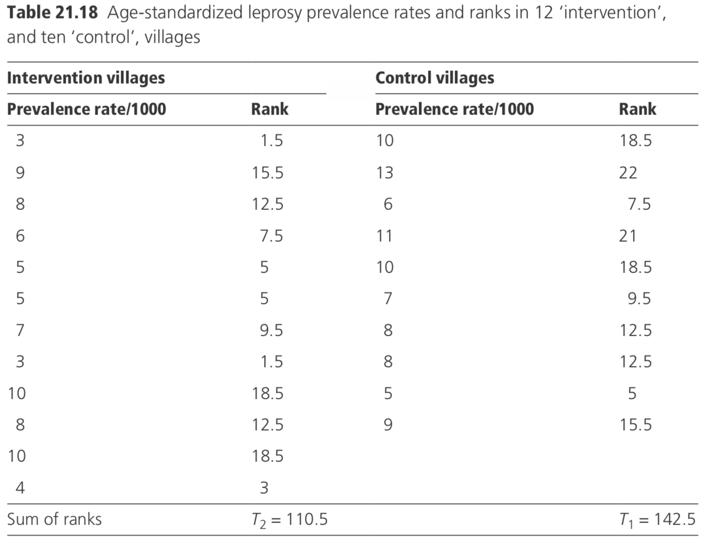
The expected value of \(T _ { 1 } = n _ { 1 } \left( n _ { 1 } + n _ { 2 } + 1 \right) / 2 = 10 ( 10 + 12 + 1 ) / 2 = 115\). As T₁ is greater than its expectation, T¹ is \(10 ( 10 + 12 + 1 ) - 142.5 = 87.5\). The critical value of T¹ at the 5% level of significance is 84 (from tables in Armitage and Berry, 1987). As T¹ is greater than the critical value, it is concluded that the intervention has not had a statistically significant effect (the average prevalence was 6.5 per thousand in intervention villages, and 8.7 per thousand in control villages).

8.3 Tests on paired data

In some study designs, communities may be ‘paired’ on the basis of similarity, with respect to confounding variables and baseline disease prevalence or incidence rates. Within each pair of communities, one receives the intervention and the other serves as the control. If this has been done, the analysis should take the pairing into account.

First, standardized response rates are computed for each community (as discussed in Section 8.1), and then the standardized response rates are compared using a paired t-test (Armitage and Berry, 1987) or a non-parametric test.

To perform a paired t-test for n pairs of communities, suppose di is the difference in outcome measured between the intervention and control unit for the i th pair. Calculate a test statistic \(\left( \Sigma d _ { \mathrm { i } } / n \right) / ( s / \sqrt { n } )\) where s is the standard deviation of the n differences. This value of the test statistic may be compared to tabulated values of the t-distribution with (n − 1) df.

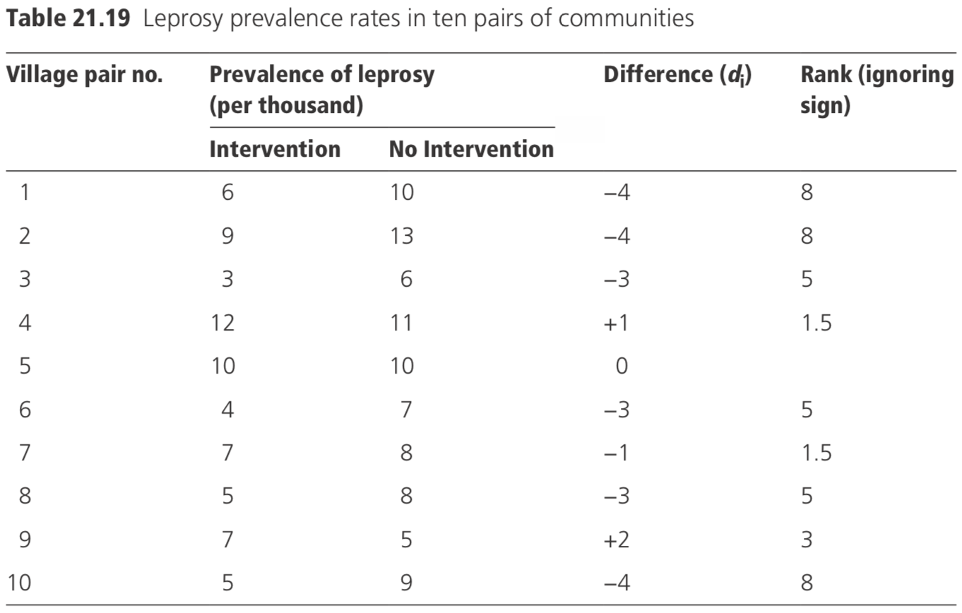
Consider the data shown in Table 21.19, which shows leprosy prevalence rates in ten pairs of communities.

The mean difference \(d = - 19 / 10 = - 1.9\), and the standard deviation of the difference (s) is 2.23. Thus, the test statistic=\(−1.9/(2.23/√10)=−2.69\) with 9 df. From tables of the t-distribution, p is <0.05, and it may be concluded that the prevalence of leprosy is significantly lower in the intervention villages.

Alternatively, a non-parametric test may be preferred. In this instance, the appropri- ate such test is Wilcoxon’s signed rank test.

The differences between each pair of villages are arranged in ascending order of mag- nitude of the absolute value of the differences (i.e. ignoring the sign) and given ranks 1 to n; zero values are excluded from analysis. Any group of tied ranks is allotted the mid rank of the group. Let:

T+ = sum of ranks of positive differences

T− = sum of ranks of negative differences.

The smaller of the two (T+ and T−) is compared with the tabulated critical value (see Table A9 of Armitage and Berry, 1987). If it is lower than the tabulated value, it is concluded that there is a significant difference. For the data in the table, \(T+ = 4.5\), and \(T− = 40.5; n = 9 \)(excluding one zero difference). The tabulated critical 5% value is 5. Since \(T+ = 4.5\) is less than 5, it is concluded that the difference is significant at the 5% level.