2.3: Dynamics of Integration- Excitation vs. Inhibition and Leak

The process of integrating the three different types of input signals (excitation, inhibition, leak) lies at the heart of neural computation. This section provides a conceptual, intuitive understanding of this process, and how it relates to the underlying electrical properties of neurons. Later, we'll see how to translate this process into mathematical equations that can actually be simulated on the computer.

Figure \(2.3\): The neuron is a tug-of-war battleground between inhibition and excitation -- the relative strength of each is what determines the membrane potential, Vm, which is what must get over threshold to fire an action potential output from the neuron.

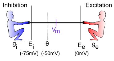
The integration process can be understood in terms of a tug-of-war (Figure 2.3). This tug-of-war takes place in the space of electrical potentials that exist in the neuron relative to the surrounding extracellular medium in which neurons live (interestingly, this medium, and the insides of neurons and other cells as well, is basically salt water with sodium (Na+), chloride (Cl-) and other ions floating around -- we carry our remote evolutionary environment around within us at all times). The core function of a neuron can be understood entirely in electrical terms: voltages (electrical potentials) and currents (flow of electrically charged ions in and out of the neuron through tiny pores called ion channels).

To see how this works, let's just consider excitation versus inhibition (inhibition and leak are effectively the same for our purposes at this time). The key point is that the integration process reflects the relative strength of excitation versus inhibition -- if excitation is stronger than inhibition, then the neuron's electrical potential (voltage) increases, perhaps to the point of getting over threshold and firing an output action potential. If inhibition is stronger, then the neuron's electrical potential decreases, and thus moves further away from getting over the threshold for firing.

Before we consider specific cases, let's introduce some obscure terminology that neuroscientists use to label the various actors in our tug-of-war drama (going from left to right in the Figure):

• -- the inhibitory conductance (g is the symbol for a conductance, and i indicates inhibition) -- this is the total strength of the inhibitory input (i.e., how strong the inhibitory guy is tugging), and plays a major role in determining how strong of an inhibitory current there is. This corresponds biologically to the proportion of inhibitory ion channels that are currently open and allowing inhibitory ions to flow (these are chloride or Cl- ions in the case of GABA inhibition, and potassium or K+ ions in the case of leak currents). For electricity buffs, the conductance is the inverse of resistance -- most people find conductance more intuitive than resistance, so we'll stick with it.
• -- the inhibitory driving potential -- in the tug-of-war metaphor, this just amounts to where the inhibitory guy happens to be standing relative to the electrical potential scale that operates within the neuron. Typically, this value is around -75mV where mV stands for millivolts -- one thousandth (1/1,000) of a volt. These are very small electrical potentials for very small neurons.
• -- the action potential threshold -- this is the electrical potential at which the neuron will fire an action potential output to signal other neurons. This is typically around -50mV. This is also called the firing threshold or the spiking threshold, because neurons are described as "firing a spike" when they get over this threshold.
• -- the membrane potential of the neuron (V = voltage or electrical potential, and m = membrane). This is the current electrical potential of the neuron relative to the extracellular space outside the neuron. It is called the membrane potential because it is the cell membrane (thin layer of fat basically) that separates the inside and outside of the neuron, and that is where the electrical potential really happens. An electrical potential or voltage is a relative comparison between the amount of electric charge in one location versus another. It is called a "potential" because when there is a difference, there is the potential to make stuff happen. For example, when there is a big potential difference between the charge in a cloud and that on the ground, it creates the potential for lightning. Just like water, differences in charge always flow "downhill" to try to balance things out. So if you have a lot of charge (water) in one location, it will flow until everything is all level. The cell membrane is effectively a dam against this flow, enabling the charge inside the cell to be different from that outside the cell. The ion channels in this context are like little tunnels in the dam wall that allow things to flow in a controlled manner. And when things flow, the membrane potential changes! In the tug-of-war metaphor, think of the membrane potential as the flag attached to the rope that marks where the balance of tugging is at the current moment.
• -- the excitatory driving potential -- this is where the excitatory guy is standing in the electrical potential space (typically around 0 mV).
• -- the excitatory conductance -- this is the total strength of the excitatory input, reflecting the proportion of excitatory ion channels that are open (these channels pass sodium or Na+ ions -- our deepest thoughts are all just salt water moving around).

Figure \(2.4\): Specific cases in the tug-of-war scenario.

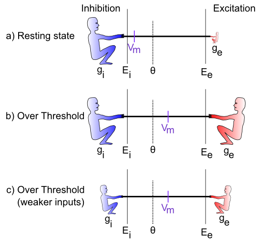is very low (indicated by the small size of the excitatory guy), which represents a neuron at rest, not receiving many excitatory input signals from other neurons. In this case, the inhibition/leak pulls much more strongly, and keeps the membrane potential (Vm) down near the -70mV territory, which is also called the resting potential of the neuron. As such, it is below the action potential threshold , and so the neuron does not output any signals itself. Everyone is just chillin'.

Figure 2.4b), the excitation is as strong as the inhibition, and this means that it can pull the membrane potential up to about the middle of the range. Because the firing threshold is toward the lower-end of the range, this is enough to get over threshold and fire a spike! The neuron will now communicate its signal to other neurons, and contribute to the overall flow of information in the brain's network.

The last case (Figure 2.4c) is particularly interesting, because it illustrates that the integration process is fundamentally relative -- what matters is how strong excitation is relative to the inhibition. If both are overall weaker, then neurons can still get over firing threshold. Can you think of any real-world example where this might be important? Consider the neurons in your visual system, which can experience huge variation in the overall amount of light coming into them depending on what you're looking at (e.g., compare snowboarding on a bright sunny day versus walking through thick woods after sunset). It turns out that the total amount of light coming into the visual system drives both a "background" level of inhibition, in addition to the amount of excitation that visual neurons experience. Thus, when it's bright, neurons get greater amounts of both excitation and inhibition compared to when it is dark. This enables the neurons to remain in their sensitive range for detecting things despite large differences in overall input levels.