7.3: Dopamine and Temporal Difference Reinforcement Learning
- Page ID
- 12605
\( \newcommand{\vecs}[1]{\overset { \scriptstyle \rightharpoonup} {\mathbf{#1}} } \)
\( \newcommand{\vecd}[1]{\overset{-\!-\!\rightharpoonup}{\vphantom{a}\smash {#1}}} \)
\( \newcommand{\id}{\mathrm{id}}\) \( \newcommand{\Span}{\mathrm{span}}\)
( \newcommand{\kernel}{\mathrm{null}\,}\) \( \newcommand{\range}{\mathrm{range}\,}\)
\( \newcommand{\RealPart}{\mathrm{Re}}\) \( \newcommand{\ImaginaryPart}{\mathrm{Im}}\)
\( \newcommand{\Argument}{\mathrm{Arg}}\) \( \newcommand{\norm}[1]{\| #1 \|}\)
\( \newcommand{\inner}[2]{\langle #1, #2 \rangle}\)
\( \newcommand{\Span}{\mathrm{span}}\)
\( \newcommand{\id}{\mathrm{id}}\)
\( \newcommand{\Span}{\mathrm{span}}\)
\( \newcommand{\kernel}{\mathrm{null}\,}\)
\( \newcommand{\range}{\mathrm{range}\,}\)
\( \newcommand{\RealPart}{\mathrm{Re}}\)
\( \newcommand{\ImaginaryPart}{\mathrm{Im}}\)
\( \newcommand{\Argument}{\mathrm{Arg}}\)
\( \newcommand{\norm}[1]{\| #1 \|}\)
\( \newcommand{\inner}[2]{\langle #1, #2 \rangle}\)
\( \newcommand{\Span}{\mathrm{span}}\) \( \newcommand{\AA}{\unicode[.8,0]{x212B}}\)
\( \newcommand{\vectorA}[1]{\vec{#1}} % arrow\)
\( \newcommand{\vectorAt}[1]{\vec{\text{#1}}} % arrow\)
\( \newcommand{\vectorB}[1]{\overset { \scriptstyle \rightharpoonup} {\mathbf{#1}} } \)
\( \newcommand{\vectorC}[1]{\textbf{#1}} \)
\( \newcommand{\vectorD}[1]{\overrightarrow{#1}} \)
\( \newcommand{\vectorDt}[1]{\overrightarrow{\text{#1}}} \)
\( \newcommand{\vectE}[1]{\overset{-\!-\!\rightharpoonup}{\vphantom{a}\smash{\mathbf {#1}}}} \)
\( \newcommand{\vecs}[1]{\overset { \scriptstyle \rightharpoonup} {\mathbf{#1}} } \)
\( \newcommand{\vecd}[1]{\overset{-\!-\!\rightharpoonup}{\vphantom{a}\smash {#1}}} \)
\(\newcommand{\avec}{\mathbf a}\) \(\newcommand{\bvec}{\mathbf b}\) \(\newcommand{\cvec}{\mathbf c}\) \(\newcommand{\dvec}{\mathbf d}\) \(\newcommand{\dtil}{\widetilde{\mathbf d}}\) \(\newcommand{\evec}{\mathbf e}\) \(\newcommand{\fvec}{\mathbf f}\) \(\newcommand{\nvec}{\mathbf n}\) \(\newcommand{\pvec}{\mathbf p}\) \(\newcommand{\qvec}{\mathbf q}\) \(\newcommand{\svec}{\mathbf s}\) \(\newcommand{\tvec}{\mathbf t}\) \(\newcommand{\uvec}{\mathbf u}\) \(\newcommand{\vvec}{\mathbf v}\) \(\newcommand{\wvec}{\mathbf w}\) \(\newcommand{\xvec}{\mathbf x}\) \(\newcommand{\yvec}{\mathbf y}\) \(\newcommand{\zvec}{\mathbf z}\) \(\newcommand{\rvec}{\mathbf r}\) \(\newcommand{\mvec}{\mathbf m}\) \(\newcommand{\zerovec}{\mathbf 0}\) \(\newcommand{\onevec}{\mathbf 1}\) \(\newcommand{\real}{\mathbb R}\) \(\newcommand{\twovec}[2]{\left[\begin{array}{r}#1 \\ #2 \end{array}\right]}\) \(\newcommand{\ctwovec}[2]{\left[\begin{array}{c}#1 \\ #2 \end{array}\right]}\) \(\newcommand{\threevec}[3]{\left[\begin{array}{r}#1 \\ #2 \\ #3 \end{array}\right]}\) \(\newcommand{\cthreevec}[3]{\left[\begin{array}{c}#1 \\ #2 \\ #3 \end{array}\right]}\) \(\newcommand{\fourvec}[4]{\left[\begin{array}{r}#1 \\ #2 \\ #3 \\ #4 \end{array}\right]}\) \(\newcommand{\cfourvec}[4]{\left[\begin{array}{c}#1 \\ #2 \\ #3 \\ #4 \end{array}\right]}\) \(\newcommand{\fivevec}[5]{\left[\begin{array}{r}#1 \\ #2 \\ #3 \\ #4 \\ #5 \\ \end{array}\right]}\) \(\newcommand{\cfivevec}[5]{\left[\begin{array}{c}#1 \\ #2 \\ #3 \\ #4 \\ #5 \\ \end{array}\right]}\) \(\newcommand{\mattwo}[4]{\left[\begin{array}{rr}#1 \amp #2 \\ #3 \amp #4 \\ \end{array}\right]}\) \(\newcommand{\laspan}[1]{\text{Span}\{#1\}}\) \(\newcommand{\bcal}{\cal B}\) \(\newcommand{\ccal}{\cal C}\) \(\newcommand{\scal}{\cal S}\) \(\newcommand{\wcal}{\cal W}\) \(\newcommand{\ecal}{\cal E}\) \(\newcommand{\coords}[2]{\left\{#1\right\}_{#2}}\) \(\newcommand{\gray}[1]{\color{gray}{#1}}\) \(\newcommand{\lgray}[1]{\color{lightgray}{#1}}\) \(\newcommand{\rank}{\operatorname{rank}}\) \(\newcommand{\row}{\text{Row}}\) \(\newcommand{\col}{\text{Col}}\) \(\renewcommand{\row}{\text{Row}}\) \(\newcommand{\nul}{\text{Nul}}\) \(\newcommand{\var}{\text{Var}}\) \(\newcommand{\corr}{\text{corr}}\) \(\newcommand{\len}[1]{\left|#1\right|}\) \(\newcommand{\bbar}{\overline{\bvec}}\) \(\newcommand{\bhat}{\widehat{\bvec}}\) \(\newcommand{\bperp}{\bvec^\perp}\) \(\newcommand{\xhat}{\widehat{\xvec}}\) \(\newcommand{\vhat}{\widehat{\vvec}}\) \(\newcommand{\uhat}{\widehat{\uvec}}\) \(\newcommand{\what}{\widehat{\wvec}}\) \(\newcommand{\Sighat}{\widehat{\Sigma}}\) \(\newcommand{\lt}{<}\) \(\newcommand{\gt}{>}\) \(\newcommand{\amp}{&}\) \(\definecolor{fillinmathshade}{gray}{0.9}\)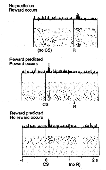
Although we considered above how phasic changes in dopamine can drive Go and NoGo learning to select the most rewarding actions and to avoid less rewarding ones, we have not addressed above how dopamine neurons come to represent these phasic signals for driving learning. One of the most exciting discoveries in recent years was the finding that dopamine neurons in the ventral tegmental area (VTA) and substantia nigra pars compacta (SNc) behave in accord with reinforcement learning models based on reward prediction error. Unlike some popular misconceptions, these dopamine neurons do not encode raw reward value directly. Instead, they encode the difference between reward received versus an expectation of reward. This is shown in Figure 7.5: if there is no expectation of reward, then dopamine neurons fire to the reward, reflecting a positive reward prediction error (zero expectation, positive reward). If a conditioned stimulus (CS, e.g., a tone or light) reliably predicts a subsequent reward, then the neurons no longer fire to the reward itself, reflecting the lack of reward prediction error (expectation = reward). Instead, the dopamine neurons fire to the onset of the CS. If the reward is omitted following the CS, then the dopamine neurons actually go the other way (a "dip" or "pause" in the otherwise low tonic level of dopamine neuron firing), reflecting a negative reward prediction error (positive reward prediction, zero reward).
Computationally, the simplest model of reward prediction error is the Rescorla-Wagner conditioning model, which is mathematically identical to the delta rule as discussed in the Learning Mechanisms chapter, and is simply the difference between the actual reward and the expected reward:
- \(\delta=r-\hat{r}\)
- \(\delta=r-\sum x w\)
where \(\delta\) ("delta") is the reward prediction error, r is the amount of reward actually received, and \(\hat{r}=\sum x w\) is the amount of reward expected, which is computed as a weighted sum over input stimuli \(x\) with weights \(w\). The weights adapt to try to accurately predict the actual reward values, and in fact this delta value specifies the direction in which the weights should change:
- \(\Delta w=\delta x\)
This is identical to the delta learning rule, including the important dependence on the stimulus activity \(x\) -- you only want to change the weights for stimuli that are actually present (i.e., non-zero \(x\)'s).
When the reward prediction is correct, then the actual reward value is cancelled out by the prediction, as shown in the second panel in Figure 7.5. This rule also accurately predicts the other cases shown in the figure too (positive and negative reward prediction errors).
What the Rescorla-Wagner model fails to capture is the firing of dopamine to the onset of the CS in the second panel in Figure 7.5. However, a slightly more complex model known as the temporal differences (TD) learning rule does capture this CS-onset firing, by introducing time into the equation (as the name suggests). Relative to Rescorla-Wagner, TD just adds one additional term to the delta equation, representing the future reward values that might come later in time:
- \(\delta=(r+f)-\hat{r}\)
where \(f\) represents the future rewards, and now the reward expectation \(\hat{r}=\sum x w\) has to try to anticipate both the current reward \(r\) and this future reward \(f\). In a simple conditioning task, where the CS reliably predicts a subsequent reward, the onset of the CS results in an increase in this \(f\) value, because once the CS arrives, there is a high probability of reward in the near future. Furthermore, this \(f\) itself is not predictable, because the onset of the CS is not predicted by any earlier cue (and if it was, then that earlier cue would be the real CS, and drive the dopamine burst). Therefore, the \(\hat{r}\) expectation cannot cancel out the \(f\) value, and a dopamine burst ensues.
Although this \(f\) value explains CS-onset dopamine firing, it raises the question of how can the system know what kind of rewards are coming in the future? Like anything having to do with the future, you fundamentally just have to guess, using the past as your guide as best as possible. TD does this by trying to enforce consistency in reward estimates over time. In effect, the estimate at time \(t\) is used to train the estimate at time \(t-1\), and so on, to keep everything as consistent as possible across time, and consistent with the actual rewards that are received over time.
This can all be derived in a very satisfying way by specifying something known as a value function, V(t) that is a sum of all present and future rewards, with the future rewards discounted by a "gamma" factor, which captures the intuitive notion that rewards further in the future are worth less than those that will occur sooner. As the Wimpy character says in Popeye, "I'll gladly pay you Tuesday for a hamburger today." Here is that value function, which is an infinite sum going into the future:
- \(V(t)=r(t)+\gamma^{1} r(t+1)+\gamma^{2} r(t+2) \ldots\)
We can get rid of the infinity by writing this equation recursively:
- \(V(t)=r(t)+\gamma V(t+1)\)
And because we don't know anything for certain, all of these value terms are really estimates, denoted by the little "hats" above them:
- \(\hat{V}(t)=r(t)+\gamma \hat{V}(t+1)\)
So this equation tells us what our estimate at the current time \(t\) should be, in terms of the future estimate at time \(t+1\). Next, we subtract \(\hat{V}\) from both sides, which gives us an expression that is another way of expressing the above equality -- that the difference between these terms should be equal to zero:
- \(0=(r(t)+\hat{V}(t+1))-\hat{V}(t)\)
This is mathematically stating the point that TD tries to keep the estimates consistent over time -- their difference should be zero. But as we are learning our \(\hat{V}\) estimates, this difference will not be zero, and in fact, the extent to which it is not zero is the extent to which there is a reward prediction error:
- \(\delta=(r(t)+\hat{V}(t+1))-\hat{V}(t)\)
If you compare this to the equation with \(f\) in it above, you can see that:
- \(f=\gamma \hat{V}(t+1)\)
and otherwise everything else is the same, except we've clarified the time dependence of all the variables, and our reward expectation is now a "value expectation" instead (replacing the \(\hat{r}\) with a \(\hat{V}\)). Also, as with Rescorla-Wagner, the delta value here drives learning of the value expectations.
The TD learning rule can be used to explain a large number of different conditioning phenomena, and its fit with the firing of dopamine neurons in the brain has led to a large amount of research progress. It represents a real triumph of the computational modeling approach for understanding (and predicting) brain function.
Exploration of TD Learning
Open RL for an exploration of TD-based reinforcement learning in simple conditioning paradigms. This exploration should help solidify your understanding of reinforcement learning, reward prediction error, and simple classical conditioning.
The Actor-Critic Architecture for Motor Learning
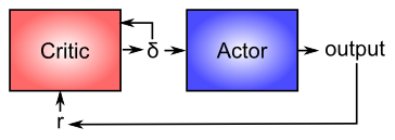
Now that you have a better idea about how dopamine works, we can revisit its role in modulating learning in the basal ganglia (as shown in Figure 7.4). From a computational perspective, the key idea is the distinction between an actor and a critic (Figure 7.6), where it is assumed that rewards result at least in part from correct performance by the actor. The basal ganglia is the actor in this case, and the dopamine signal is the output of the critic, which then serves as a training signal for the actor (and the critic too as we saw earlier). The reward prediction error signal produced by the dopamine system is a good training signal because it drives stronger learning early in a skill acquisition process, when rewards are more unpredictable, and reduces learning as the skill is perfected, and rewards are thus more predictable. If the system instead learned directly on the basis of external rewards, it would continue to learn about skills that have long been mastered, and this would likely lead to a number of bad consequences (synaptic weights growing ever stronger, interference with other newer learning, etc).
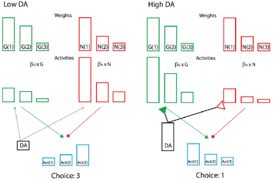
Furthermore, the sign of the reward prediction error is appropriate for the effects of dopamine on the Go and NoGo pathways in the striatum, as we saw in the BG model project above. Positive reward prediction errors, when unexpected rewards are received, indicate that the selected action was better than expected, and thus Go firing for that action should be increased in the future. The increased activation produced by dopamine on these Go neurons will have this effect, assuming learning is driven by these activation levels. Conversely, negative reward prediction errors will facilitate NoGo firing, causing the system to avoid that action in the future. Indeed, the complex neural network model of BG Go/NoGo circuitry can be simplified with more formal analysis in a modified actor-critic architecture called Opponent Actor Learning (OpAL; Figure 7.7), where the actor is divided into independent G and N opponent weights, and where their relative contribution is itself affected by dopamine levels during both learning and choice (Collins & Frank 2014).
Finally, the ability of the dopamine signal to propagate backward in time is critical for spanning the inevitable delays between motor actions and subsequent rewards. Specifically, the dopamine response should move from the time of the reward to the time of the action that reliably predicts reward, in the same way that it moves in time to the onset of the CS in a classical conditioning paradigm.
The PVLV Model of DA Biology
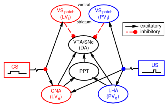
You might have noticed that we haven't yet explained at a biological level how the dopamine neurons in the VTA and SNc actually come to exhibit their reward prediction error firing. There is a growing body of data supporting the involvement of the brain areas shown in Figure 7.8:
- Lateral hypothalamus (LHA) provides a primary reward signal for basic rewards like food, water etc.
- Patch-like neurons in the ventral striatum (VS-patch) have direct inhibitory connections onto the dopamine neurons in the VTA and SNc, and likely play the role of canceling out the influence of primary reward signals when these rewards have successfully been predicted.
- Central nucleus of the amygdala (CNA) is important for driving dopamine firing to the onset of conditioned stimuli. It receives broadly from the cortex, and projects directly and indirectly to the VTA and SNc. Neurons in the CNA exhibit CS-related firing.
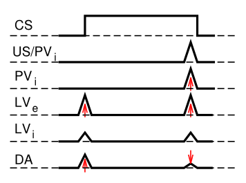
Given that there are distinct brain areas involved in these different aspects of the dopamine firing, it raises the question as to how the seemingly unified TD learning algorithm could be implemented across such different brain areas? In response to this basic question, the PVLV model of dopamine firing was developed. PVLV stands for Primary Value, Learned Value, and the key idea is that different brain structures are involved at the time when primary values are being experienced, versus when conditioned stimuli (learned values) are being experienced. This then requires a different mathematical formulation, as compared to TD.
The dopamine signal in PVLV for primary values (PV), which is in effect at the time external rewards are delivered or expected, is identical to Rescorla-Wagner, just using different labels for the variables:
- \(\delta_{p v}=r-\hat{r}\)
- \(\delta_{p v}=P V_{e}-P V_{i}\)
Where excitatory (\(e\)) and inhibitory (\(i\)) subscripts denote the two components of the primary value system, and the sign of their influence on dopamine firing.
The dopamine signal for learned values (LV) applies whenever PV does not (i.e., when external rewards are not present or expected), and it has a similar form:
- \(\delta_{l v}=L V_{e}-L V_{i}\)
Where \(L V_{e}\) is the excitatory drive on dopamine from the CNA, which learns to respond to CS's. \(L V_{i}\) is a counteracting inhibitory drive, again thought to be associated with the patch-like neurons of the ventral striatum. It learns much more slowly than the \(L V_{e}\) system, and will eventually learn to cancel out CS-associated dopamine responses, once these CS's become highly highly familiar (beyond the short timescale of most experiments).
The \(P V_{i}\) values are learned in the same way as in the delta rule or Rescorla-Wagner, and the \(L V_{e}\) and \(L V_{i}\) values are learned in a similar fashion as well, except that their training signal is driven directly from the \(P V_{e}\) reward values, and only occurs when external rewards are present or expected. This is critical for allowing \(L V_{e}\) for example to get activated at the time of CS onset, when there isn't any actual reward value present. If \(L V_{e}\) was always learning to match the current value of \(P V_{e}\), then this absence of \(P V_{e}\) value at CS onset would quickly eliminate the \(L V_{e}\) response then. See PVLV Learning for the full set of equations governing the learning of the LV and PV components.
There are a number of interesting properties of the learning constraints in the PVLV system. First, the CS must still be active at the time of the external reward in order for the \(L V_{e}\) system to learn about it, since LV only learns at the time of external reward. If the CS itself goes off, then some memory of it must be sustained. This fits well with known constraints on CS learning in conditioning paradigms. Second, the dopamine burst at the time of CS onset cannot influence learning in the LV system itself -- otherwise there would be an unchecked positive feedback loop. One implication of this is that the LV system cannot support second-order conditioning, where a first CS predicts a second CS which then predicts reward. Consistent with this constraint, the CNA (i.e., \(L V_{e}\)) appears to only be involved in first order conditioning, while the basolateral nucleus of the amygdala (BLA) is necessary for second-order conditioning. Furthermore, there does not appear to be much of any evidence for third or higher orders of conditioning. Finally, there is a wealth of specific data on differences in CS vs. US associated learning that are consistent with the PVLV framework (see Hazy et al, 2010 for a thorough review).
In short, the PVLV system can explain how the different biological systems are involved in generating phasic dopamine responses as a function of reward associations, in a way that seems to fit with otherwise somewhat peculiar constraints on the system. Also, we will see in the Executive Function Chapter that PVLV provides a cleaner learning signal for controlling the basal ganglia's role in the prefrontal cortex working memory system.
Exploration of PVLV
- PVLV model of same simple conditioning cases as explored in TD model: PVLV


