
1.5: Random Error
- Page ID
- 38518

\( \newcommand{\vecs}[1]{\overset { \scriptstyle \rightharpoonup} {\mathbf{#1}} } \)
\( \newcommand{\vecd}[1]{\overset{-\!-\!\rightharpoonup}{\vphantom{a}\smash {#1}}} \)
\( \newcommand{\dsum}{\displaystyle\sum\limits} \)
\( \newcommand{\dint}{\displaystyle\int\limits} \)
\( \newcommand{\dlim}{\displaystyle\lim\limits} \)
\( \newcommand{\id}{\mathrm{id}}\) \( \newcommand{\Span}{\mathrm{span}}\)
( \newcommand{\kernel}{\mathrm{null}\,}\) \( \newcommand{\range}{\mathrm{range}\,}\)
\( \newcommand{\RealPart}{\mathrm{Re}}\) \( \newcommand{\ImaginaryPart}{\mathrm{Im}}\)
\( \newcommand{\Argument}{\mathrm{Arg}}\) \( \newcommand{\norm}[1]{\| #1 \|}\)
\( \newcommand{\inner}[2]{\langle #1, #2 \rangle}\)
\( \newcommand{\Span}{\mathrm{span}}\)
\( \newcommand{\id}{\mathrm{id}}\)
\( \newcommand{\Span}{\mathrm{span}}\)
\( \newcommand{\kernel}{\mathrm{null}\,}\)
\( \newcommand{\range}{\mathrm{range}\,}\)
\( \newcommand{\RealPart}{\mathrm{Re}}\)
\( \newcommand{\ImaginaryPart}{\mathrm{Im}}\)
\( \newcommand{\Argument}{\mathrm{Arg}}\)
\( \newcommand{\norm}[1]{\| #1 \|}\)
\( \newcommand{\inner}[2]{\langle #1, #2 \rangle}\)
\( \newcommand{\Span}{\mathrm{span}}\) \( \newcommand{\AA}{\unicode[.8,0]{x212B}}\)
\( \newcommand{\vectorA}[1]{\vec{#1}} % arrow\)
\( \newcommand{\vectorAt}[1]{\vec{\text{#1}}} % arrow\)
\( \newcommand{\vectorB}[1]{\overset { \scriptstyle \rightharpoonup} {\mathbf{#1}} } \)
\( \newcommand{\vectorC}[1]{\textbf{#1}} \)
\( \newcommand{\vectorD}[1]{\overrightarrow{#1}} \)
\( \newcommand{\vectorDt}[1]{\overrightarrow{\text{#1}}} \)
\( \newcommand{\vectE}[1]{\overset{-\!-\!\rightharpoonup}{\vphantom{a}\smash{\mathbf {#1}}}} \)
\( \newcommand{\vecs}[1]{\overset { \scriptstyle \rightharpoonup} {\mathbf{#1}} } \)
\(\newcommand{\longvect}{\overrightarrow}\)
\( \newcommand{\vecd}[1]{\overset{-\!-\!\rightharpoonup}{\vphantom{a}\smash {#1}}} \)
\(\newcommand{\avec}{\mathbf a}\) \(\newcommand{\bvec}{\mathbf b}\) \(\newcommand{\cvec}{\mathbf c}\) \(\newcommand{\dvec}{\mathbf d}\) \(\newcommand{\dtil}{\widetilde{\mathbf d}}\) \(\newcommand{\evec}{\mathbf e}\) \(\newcommand{\fvec}{\mathbf f}\) \(\newcommand{\nvec}{\mathbf n}\) \(\newcommand{\pvec}{\mathbf p}\) \(\newcommand{\qvec}{\mathbf q}\) \(\newcommand{\svec}{\mathbf s}\) \(\newcommand{\tvec}{\mathbf t}\) \(\newcommand{\uvec}{\mathbf u}\) \(\newcommand{\vvec}{\mathbf v}\) \(\newcommand{\wvec}{\mathbf w}\) \(\newcommand{\xvec}{\mathbf x}\) \(\newcommand{\yvec}{\mathbf y}\) \(\newcommand{\zvec}{\mathbf z}\) \(\newcommand{\rvec}{\mathbf r}\) \(\newcommand{\mvec}{\mathbf m}\) \(\newcommand{\zerovec}{\mathbf 0}\) \(\newcommand{\onevec}{\mathbf 1}\) \(\newcommand{\real}{\mathbb R}\) \(\newcommand{\twovec}[2]{\left[\begin{array}{r}#1 \\ #2 \end{array}\right]}\) \(\newcommand{\ctwovec}[2]{\left[\begin{array}{c}#1 \\ #2 \end{array}\right]}\) \(\newcommand{\threevec}[3]{\left[\begin{array}{r}#1 \\ #2 \\ #3 \end{array}\right]}\) \(\newcommand{\cthreevec}[3]{\left[\begin{array}{c}#1 \\ #2 \\ #3 \end{array}\right]}\) \(\newcommand{\fourvec}[4]{\left[\begin{array}{r}#1 \\ #2 \\ #3 \\ #4 \end{array}\right]}\) \(\newcommand{\cfourvec}[4]{\left[\begin{array}{c}#1 \\ #2 \\ #3 \\ #4 \end{array}\right]}\) \(\newcommand{\fivevec}[5]{\left[\begin{array}{r}#1 \\ #2 \\ #3 \\ #4 \\ #5 \\ \end{array}\right]}\) \(\newcommand{\cfivevec}[5]{\left[\begin{array}{c}#1 \\ #2 \\ #3 \\ #4 \\ #5 \\ \end{array}\right]}\) \(\newcommand{\mattwo}[4]{\left[\begin{array}{rr}#1 \amp #2 \\ #3 \amp #4 \\ \end{array}\right]}\) \(\newcommand{\laspan}[1]{\text{Span}\{#1\}}\) \(\newcommand{\bcal}{\cal B}\) \(\newcommand{\ccal}{\cal C}\) \(\newcommand{\scal}{\cal S}\) \(\newcommand{\wcal}{\cal W}\) \(\newcommand{\ecal}{\cal E}\) \(\newcommand{\coords}[2]{\left\{#1\right\}_{#2}}\) \(\newcommand{\gray}[1]{\color{gray}{#1}}\) \(\newcommand{\lgray}[1]{\color{lightgray}{#1}}\) \(\newcommand{\rank}{\operatorname{rank}}\) \(\newcommand{\row}{\text{Row}}\) \(\newcommand{\col}{\text{Col}}\) \(\renewcommand{\row}{\text{Row}}\) \(\newcommand{\nul}{\text{Nul}}\) \(\newcommand{\var}{\text{Var}}\) \(\newcommand{\corr}{\text{corr}}\) \(\newcommand{\len}[1]{\left|#1\right|}\) \(\newcommand{\bbar}{\overline{\bvec}}\) \(\newcommand{\bhat}{\widehat{\bvec}}\) \(\newcommand{\bperp}{\bvec^\perp}\) \(\newcommand{\xhat}{\widehat{\xvec}}\) \(\newcommand{\vhat}{\widehat{\vvec}}\) \(\newcommand{\uhat}{\widehat{\uvec}}\) \(\newcommand{\what}{\widehat{\wvec}}\) \(\newcommand{\Sighat}{\widehat{\Sigma}}\) \(\newcommand{\lt}{<}\) \(\newcommand{\gt}{>}\) \(\newcommand{\amp}{&}\) \(\definecolor{fillinmathshade}{gray}{0.9}\)Learning Objectives
After reading this chapter, you will be able to do the following:
- Define random error and differentiate it from bias
- Illustrate random error with examples
- Interpret a p-value
- Interpret a confidence interval
- Differentiate between type 1 and type 2 statistical errors and explain how they apply to epidemiologic research
- Describe how statistical power affects research
In this chapter, we will cover random error—where it comes from, how we deal with it, and what it means for epidemiology.
What Is Random Error?
First and foremost, random error is not bias. Bias is systematic error and is covered in further detail in chapter 6.
Random error is just what it sounds like: random errors in the data. All data contain random errors, because no measurement system is perfect. The magnitude of random errors depends partly on the scale on which something is measured (errors in molecular-level measurements would be on the order of nanometers, whereas errors in human height measurements are probably on the order of a centimeter or two) and partly on the quality of the tools being used. Physics and chemistry labs have highly accurate, expensive scales that can measure mass to the nearest gram, microgram, or nanogram, whereas the average scale in someone’s bathroom is probably accurate within a half-pound or pound.
To wrap your head around random error, imagine that you are baking a cake that requires 6 tablespoons of butter. To get the 6 tablespoons of butter (three-quarters of a stick, if there are 4 sticks in a pound, as is usually true in the US), you could use the marks that appear on the waxed paper around the stick, assuming they are lined up correctly. Or you could perhaps follow my mother’s method, which is to unwrap the stick, make a slight mark at what looks like one-half of the stick, and then get to three-quarters by eyeballing half of the one-half. Or you could use my method, which is to eyeball the three-quarter mark from the start and slice away. Any of these “measurement” methods will give you roughly 6 tablespoons of butter, which is certainly good enough for the purposes of baking a cake—but probably not exactly 3 ounces’ worth, which is how much 6 tablespoons of butter weighs in the US.[i] The extent to which you’re slightly over 3 ounces this time and perhaps slightly under 3 ounces next time is causing random error in your measurement of butter. If you always underestimated or always overestimated, then that would be a bias—however, your consistently under- or overestimated measurements would within themselves contain random error.
Inherent Variability
For any given variable that we might want to measure in epidemiology (e.g., height, GPA, heart rate, number of years working at a particular factory, serum triglyceride level, etc.), we expect there to be variability in the sample—that is, we do not expect everyone in the population to have exactly the same value. This is not random error. Random error (and bias) occurs when we try to measure these things. Indeed, epidemiology as a field relies on this inherent variability. If everyone were exactly the same, then we would not be able to identify which kinds of people were at higher risk for developing a particular disease.
In epidemiology, sometimes our measurements rely on a human other than the study participant measuring something on or about the participant. Examples would include measured height or weight, blood pressure, or serum cholesterol. For some of these (e.g., weight and serum cholesterol), the random error creeps into the data because of the instrument being used—here, a scale that has probably a half-pound fluctuation, or a laboratory assay with a margin of error of a few milligrams per deciliter. For other measurements (e.g., height and blood pressure), the measurer themselves is responsible for any random error, as in the butter example.
However, many of our measurements rely on participant self-reporting. There are whole textbooks and classes devoted to questionnaire design, and the science behind how to get the most accurate data from people via survey methods is quite good. The Pew Research Center offers a nice introductory tutorial on questionnaire design on its website.
Relevant to our discussion here, random error will appear in questionnaire data as well. For some variables, there will be less random error than others (e.g., self-reported race is probably quite accurate), but there will still be some—for example, people accidentally checking the wrong box. For other variables, there will be more random error (e.g., imprecise answers to questions such as, “In the last year, how many times per month did you eat rice?”). A good question to ask yourself when considering the amount of random error that might be in a variable derived from a questionnaire is, “Can people tell me this?” Most people could theoretically tell you how much sleep they got last night, but they would be hard-pressed to tell you how much sleep they got on the same night one year ago. Whether or not they will tell you is a different matter and touches on bias (see chapter 6). Regardless, random error in questionnaire data increases as the likelihood that people could tell you the answer decreases.
Quantifying Random Error
While we can—and should—work to minimize random error (using high-quality instruments, training staff on how to take measurements, designing good questionnaires, etc.), it can never be eliminated entirely. Luckily, we can use statistics to quantify the random errors present in a study. Indeed, this is what statistics is for. In this book, I will cover only a small slice of the vast field of statistics: interpretation of p-values and confidence intervals (CI). Rather than focus on how to calculate them[1], I will instead focus on what they mean (and what they do not mean). Knowledge of p-values and CIs is sufficient to allow accurate interpretation of the results of epidemiologic studies for beginning epidemiology students.
p-values
When conducting scientific research of any kind, including epidemiology, one begins with a hypothesis, which is then tested as the study is conducted. For example, if we are studying average height of undergraduate students, our hypothesis (usually indicated by H1) might be that male students are, on average, taller than female students. However, for statistical testing purposes, we must rephrase our hypothesis as a null hypothesis [2]. In this case, our null hypothesis (usually indicated by H0) would be the following:
We would then undertake our study to test this hypothesis. We first determine the target population (undergraduate students) and draw a sample from this population. We then measure the heights and genders of everyone in the sample, and calculate mean height among men versus that among women. We would then conduct a statistical test to compare the mean heights in the 2 groups. Because we have a continuous variable (height) measured in 2 groups (men and women), we would use a t-test[3], and the t-statistic calculated via this test would have a corresponding p-value, which is what we really care about.
Let’s say that in our study we find that male students average 5 feet 10 inches, and among female students the mean height is 5 feet 6 inches (for a difference of 4 inches), and we calculate a p-value of 0.04. This means that if there really is no difference in average height between male students and female students (i.e., if the null hypothesis is true) and we repeat the study (all the way back to drawing a new sample from the population), there is a 4% chance that we will again find a difference in mean height of 4 inches or more.
There are several implications that stem from the above paragraph. First, in epidemiology we always calculate 2-tailed p-values. Here this simply means that the 4% chance of a ≥4 inch height difference says nothing about which group is taller—just that one group (either males or females) will be taller on average by at least 4 inches. Second, p-values are meaningless if you happen to be able to enroll the entire population in your study. As an example, say our research question pertains to students in Public Health 425 (H425, Foundations of Epidemiology) during the 2020 winter term at Oregon State University (OSU). Are men or women taller in this population? As the population is quite small and all members are easily identified, we can enroll everyone instead of having to rely on a sample. There will still be random error in the measurement of height, but we no longer use a p-value to quantify it. This is because if we were to repeat the study, we would find exactly the same thing, since we actually measured everyone in the population. P-values only apply if we are working with samples.
Finally, note that the p-value describes the probability of your data, assuming the null hypothesis is true—it does not describe the probability of the null hypothesis being true given your data. This is a common interpretation mistake made by both beginning and senior readers of epidemiologic studies. The p-value says nothing about how likely it is that the null hypothesis is true (and thus on the flip side, about the truth of your actual hypothesis). Rather, it quantifies the likelihood of getting the data that you got if the null hypothesis did happen to be true. This is a subtle distinction but a very important one.
Statistical Significance
What happens next? We have a p-value, which tells us the chance of getting our data given the null hypothesis. But what does that actually mean in terms of what to conclude about a study’s results? In public health and clinical research, the standard practice is to use p ≤ 0.05 to indicate statistical significance. In other words, decades of researchers in this field have collectively decided that if the chance of committing a type I error (more on that below) is 5% or less, we will “reject the null hypothesis.” Continuing height example from above, we would thus conclude that there is a difference in height between genders, at least among undergraduate students. For p-values above 0.05, we “fail to reject the null hypothesis,” and instead conclude that our data provided no evidence that there was a difference in height between male and female undergraduate students.
Failing to Reject the Null vs. Accepting the Null
If p > 0.05, we fail to reject the null hypothesis. We do not ever accept the null hypothesis because it is very difficult to prove the absence of something. “Accepting” the null hypothesis implies that we have proven that there really is no difference in height between male and female students, which is not what happened. If p > 0.05, it merely means that we did not find evidence in opposition to the null hypothesis—not that said evidence doesn’t exist. We might have gotten a weird sample, we might have had too small a sample, etc. There is a whole field of clinical research (comparative effectiveness researchvi) dedicated to showing that one treatment is no better or worse than another; the field’s methods are complex, and the sample sizes required are quite large. For most epidemiologic studies, we simply stick to failing to reject.
Is the p ≤ 0.05 cutoff arbitrary? Absolutely. This is worth keeping in mind, particularly for p-values very near this cutoff. Is 0.49 really that different from 0.51? Likely not, but they are on opposite sides of that arbitrary line. The size of a p-value depends on 3 things: the sample size, the effect size (it is easier to reject the null hypothesis if the true difference in height—were we to measure everyone in the population, rather than only our sample—is 6 inches rather than 2 inches), and the consistency of the data, most commonly measured by the standard deviations around the mean heights in the 2 groups. Thus a p-value of 0.51 could almost certainly be made smaller by simply enrolling more people in the study (this pertains to power, which is the inverse of type II error, discussed below). It is important to keep this fact in mind when you read studies.
Frequentist versus Bayesian Statistics
Statistical significance testing is part of a branch of statistics referred to as frequentist statistics.ii Though extremely common in epidemiology and related fields, this practice is not generally regarded as an ideal science, for a number of reasons. First and foremost, the 0.05 cutoff is entirely arbitrary,iii and strict significance testing would reject the null for p = 0.049 but fail to reject for p = 0.051, even though they are nearly identical. Second, there are many more nuances to interpretation of p-values and confidence intervals than those I have covered in this chapter.iv For instance, the p-value is really testing all analysis assumptions, not just the null hypothesis, and a large p-value often indicates merely that the data cannot discriminate among numerous competing hypotheses. However, since public health and clinical medicine both require yes-or-no decisions (Should we spend resources on that health education campaign? Should this patient get this medication?), there needs to be some system for deciding yay or nay, and statistical significance testing is currently it. There are other ways of quantifying random error, and indeed Bayesian statistics (which instead of a yes-or-no answer yields a probability of something happening)ii is becoming more and more popular. Nonetheless, as frequentist statistics and null hypothesis testing are still by far the most common methods used in epidemiologic literature, they are the focus of this chapter.
Type I and Type II errors
A type I error (usually symbolized by α, the Greek letter alpha, and closely related to p-values) is the probability that you incorrectly reject the null hypothesis – in other words, that you “find” something that’s not really there. By choosing 0.05 as our statistical significance cut-off, we in the public health and clinical research fields have tacitly agreed that we are willing to accept that 5% of our findings will really be type I errors, or false positives.
A type II error (usually symbolized by β, the Greek letter beta) is the opposite: β is the probability that you incorrectly fail to reject the null hypothesis—in other words, you miss something that really is there.
Power = 1 – β and is interpreted as the likelihood that you’ll find things if they are there.
Power in epidemiologic studies varies widely: ideally it should be at least 90% (meaning the type II error rate is 10%), but often it is much lower. Power is proportional to sample size but in an exponential manner—power goes up as sample size goes up, but to get from 90 to 95% power requires a much larger jump in sample size than to go from 40 to 45% power. If a study fails to reject the null hypothesis, but the data look like there might be a large difference between groups, often the issue is that the study was underpowered, and with a larger sample, the p-value would probably fall below the magic 0.05 cutoff. On the other hand, part of the issue with small samples is that you might just by chance have gotten a non-representative sample, and adding additional participants would not drive the results toward statistical significance. As an example, suppose we are again interested in gender-based height differences, but this time only among collegiate athletes. We begin with a very small study—just one men’s team and one women’s team. If we happen to choose, say, the men’s basketball team and the women’s gymnastics team, we are likely to find a whopping difference in mean heights—perhaps 18 inches or more. Adding other teams to our study would almost certainly result in a much narrower difference in mean heights, and the 18 inch difference “found” in our initial small study would not hold up over time.
Confidence Intervals
Because we have set the acceptable  level at 5%, in epidemiology and related fields, we most commonly use 95% confidence intervals (95% CI). One can use a 95% CI to do significance testing: if the 95% CI does not include the null value (0 for risk difference and 1.0 for odds ratios, risk ratios, and rate ratios), then p < 0.05, and the result is statistically significant.
Though 95% CI can be used for significance testing, they contain much more information than just whether the p-value is <0.05 or not. Most epidemiologic studies report 95% CI around any point estimates that are presented. The correct interpretation of a 95% CI is as follows:
If you repeated the study 100 times (back to drawing your sample from the population), and the study is free of all bias, then 95 of those 100 times the CI that you calculate would include the “real” answer that you would get were you able to enroll everyone in the population.
We can also illustrate this visually:
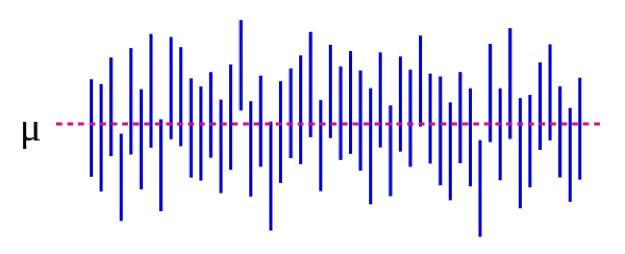
In Figure 5-1, the population parameter μ represents the “real” answer that you would get if you could enroll absolutely everyone in the population in the study. We estimate μ with data from our sample. Continuing with our height example, this might be 5 inches: if we could magically measure the heights of every single undergraduate student in the US (or the world, depending on how you defined your target population), the mean difference between male and female students would be 5 inches. Importantly, this population parameter is almost always unobservable—it only becomes observable if you define your population narrowly enough that you can enroll everyone. Each blue vertical line represents the CI of an individual “study”—50 of them, in this case. The CIs vary because the sample is slightly different each time—however, most of the CIs (all but 3, in fact) do contain μ.
If we conduct our study and find a mean difference of 4 inches (95% CI, 1.5 – 7), the CI tells us 2 things. First, the p-value for our t-test would be <0.05, since the CI excludes 0 (the null value in this case, as we are calculating a difference measure). Second, the interpretation of the CI is: if we repeated our study (including drawing a new sample) 100 times, then 95 of those times our CI would include the real value (which we know here is 5 inches, but which in real life you would not know). Thus looking at the CI here of 1.5 – 7.0 inches gives an idea of what the real difference might be—it almost certainly lies somewhere within that range but could be as small as 1.5 inches or as large as 7 inches. Like p-values, CIs depend on sample size. A large sample will yield a comparatively narrower CI. Narrower CIs are considered to be better because they yield a more precise estimate of what the “true” answer might be.
Summary
Random error is present in all measurements, though some variables are more prone to it than others. P-values and CIs are used to quantify random error. A p-value of 0.05 or less is usually taken to be “statistically significant,” and the corresponding CI would exclude the null value. CIs are useful for expressing the potential range of the “real” population-level value being estimated.
References
i. Butter in the US and the rest of the world. Errens Kitchen. March 2014. https://www.errenskitchen.com/cookin...t-conversions/. Accessed September 26, 2018. (↵ Return)
ii. Bayesian vs frequentist approach: same data, opposite results. 365 Data Sci. August 2017. https://365datascience.com/bayesian-...tist-approach/. Accessed October 17, 2018. (↵ Return 1) (↵ Return 2)
iii. Smith RJ. The continuing misuse of null hypothesis significance testing in biological anthropology. Am J Phys Anthropol. 2018;166(1):236-245. doi:10.1002/ajpa.23399 (↵ Return)
iv. Farland LV, Correia KF, Wise LA, Williams PL, Ginsburg ES, Missmer SA. P-values and reproductive health: what can clinical researchers learn from the American Statistical Association? Hum Reprod Oxf Engl. 2016;31(11):2406-2410. doi:10.1093/humrep/dew192 (↵ Return)
v. Greenland S, Senn SJ, Rothman KJ, et al. Statistical tests, p values, confidence intervals, and power: a guide to misinterpretations. Eur J Epidemiol. 2016;31:337-350. doi:10.1007/s10654-016-0149-3
vi. Why is comparative effectiveness research important? Patient-Centered Outcomes Research Institute. https://www.pcori.org/files/why-comp...arch-important. Accessed October 17, 2018. (↵ Return)
- There isn’t just one formula for calculating a p-value or a CI. Rather, the formulas change depending on which statistical test is being applied. Any introductory biostatistics text that discusses which statistical methods to use and when would also provide the corresponding information on p-value and CI calculation. ↵
- Don’t spend too long trying to figure out why we need a null hypothesis; we just do. The rationale is buried in centuries of academic philosophy of science arguments. ↵
- How to choose the correct test is beyond the scope of this book—see any book on introductory biostatistics ↵