
1.8: Effect Modification
- Page ID
- 38521

\( \newcommand{\vecs}[1]{\overset { \scriptstyle \rightharpoonup} {\mathbf{#1}} } \)
\( \newcommand{\vecd}[1]{\overset{-\!-\!\rightharpoonup}{\vphantom{a}\smash {#1}}} \)
\( \newcommand{\dsum}{\displaystyle\sum\limits} \)
\( \newcommand{\dint}{\displaystyle\int\limits} \)
\( \newcommand{\dlim}{\displaystyle\lim\limits} \)
\( \newcommand{\id}{\mathrm{id}}\) \( \newcommand{\Span}{\mathrm{span}}\)
( \newcommand{\kernel}{\mathrm{null}\,}\) \( \newcommand{\range}{\mathrm{range}\,}\)
\( \newcommand{\RealPart}{\mathrm{Re}}\) \( \newcommand{\ImaginaryPart}{\mathrm{Im}}\)
\( \newcommand{\Argument}{\mathrm{Arg}}\) \( \newcommand{\norm}[1]{\| #1 \|}\)
\( \newcommand{\inner}[2]{\langle #1, #2 \rangle}\)
\( \newcommand{\Span}{\mathrm{span}}\)
\( \newcommand{\id}{\mathrm{id}}\)
\( \newcommand{\Span}{\mathrm{span}}\)
\( \newcommand{\kernel}{\mathrm{null}\,}\)
\( \newcommand{\range}{\mathrm{range}\,}\)
\( \newcommand{\RealPart}{\mathrm{Re}}\)
\( \newcommand{\ImaginaryPart}{\mathrm{Im}}\)
\( \newcommand{\Argument}{\mathrm{Arg}}\)
\( \newcommand{\norm}[1]{\| #1 \|}\)
\( \newcommand{\inner}[2]{\langle #1, #2 \rangle}\)
\( \newcommand{\Span}{\mathrm{span}}\) \( \newcommand{\AA}{\unicode[.8,0]{x212B}}\)
\( \newcommand{\vectorA}[1]{\vec{#1}} % arrow\)
\( \newcommand{\vectorAt}[1]{\vec{\text{#1}}} % arrow\)
\( \newcommand{\vectorB}[1]{\overset { \scriptstyle \rightharpoonup} {\mathbf{#1}} } \)
\( \newcommand{\vectorC}[1]{\textbf{#1}} \)
\( \newcommand{\vectorD}[1]{\overrightarrow{#1}} \)
\( \newcommand{\vectorDt}[1]{\overrightarrow{\text{#1}}} \)
\( \newcommand{\vectE}[1]{\overset{-\!-\!\rightharpoonup}{\vphantom{a}\smash{\mathbf {#1}}}} \)
\( \newcommand{\vecs}[1]{\overset { \scriptstyle \rightharpoonup} {\mathbf{#1}} } \)
\(\newcommand{\longvect}{\overrightarrow}\)
\( \newcommand{\vecd}[1]{\overset{-\!-\!\rightharpoonup}{\vphantom{a}\smash {#1}}} \)
\(\newcommand{\avec}{\mathbf a}\) \(\newcommand{\bvec}{\mathbf b}\) \(\newcommand{\cvec}{\mathbf c}\) \(\newcommand{\dvec}{\mathbf d}\) \(\newcommand{\dtil}{\widetilde{\mathbf d}}\) \(\newcommand{\evec}{\mathbf e}\) \(\newcommand{\fvec}{\mathbf f}\) \(\newcommand{\nvec}{\mathbf n}\) \(\newcommand{\pvec}{\mathbf p}\) \(\newcommand{\qvec}{\mathbf q}\) \(\newcommand{\svec}{\mathbf s}\) \(\newcommand{\tvec}{\mathbf t}\) \(\newcommand{\uvec}{\mathbf u}\) \(\newcommand{\vvec}{\mathbf v}\) \(\newcommand{\wvec}{\mathbf w}\) \(\newcommand{\xvec}{\mathbf x}\) \(\newcommand{\yvec}{\mathbf y}\) \(\newcommand{\zvec}{\mathbf z}\) \(\newcommand{\rvec}{\mathbf r}\) \(\newcommand{\mvec}{\mathbf m}\) \(\newcommand{\zerovec}{\mathbf 0}\) \(\newcommand{\onevec}{\mathbf 1}\) \(\newcommand{\real}{\mathbb R}\) \(\newcommand{\twovec}[2]{\left[\begin{array}{r}#1 \\ #2 \end{array}\right]}\) \(\newcommand{\ctwovec}[2]{\left[\begin{array}{c}#1 \\ #2 \end{array}\right]}\) \(\newcommand{\threevec}[3]{\left[\begin{array}{r}#1 \\ #2 \\ #3 \end{array}\right]}\) \(\newcommand{\cthreevec}[3]{\left[\begin{array}{c}#1 \\ #2 \\ #3 \end{array}\right]}\) \(\newcommand{\fourvec}[4]{\left[\begin{array}{r}#1 \\ #2 \\ #3 \\ #4 \end{array}\right]}\) \(\newcommand{\cfourvec}[4]{\left[\begin{array}{c}#1 \\ #2 \\ #3 \\ #4 \end{array}\right]}\) \(\newcommand{\fivevec}[5]{\left[\begin{array}{r}#1 \\ #2 \\ #3 \\ #4 \\ #5 \\ \end{array}\right]}\) \(\newcommand{\cfivevec}[5]{\left[\begin{array}{c}#1 \\ #2 \\ #3 \\ #4 \\ #5 \\ \end{array}\right]}\) \(\newcommand{\mattwo}[4]{\left[\begin{array}{rr}#1 \amp #2 \\ #3 \amp #4 \\ \end{array}\right]}\) \(\newcommand{\laspan}[1]{\text{Span}\{#1\}}\) \(\newcommand{\bcal}{\cal B}\) \(\newcommand{\ccal}{\cal C}\) \(\newcommand{\scal}{\cal S}\) \(\newcommand{\wcal}{\cal W}\) \(\newcommand{\ecal}{\cal E}\) \(\newcommand{\coords}[2]{\left\{#1\right\}_{#2}}\) \(\newcommand{\gray}[1]{\color{gray}{#1}}\) \(\newcommand{\lgray}[1]{\color{lightgray}{#1}}\) \(\newcommand{\rank}{\operatorname{rank}}\) \(\newcommand{\row}{\text{Row}}\) \(\newcommand{\col}{\text{Col}}\) \(\renewcommand{\row}{\text{Row}}\) \(\newcommand{\nul}{\text{Nul}}\) \(\newcommand{\var}{\text{Var}}\) \(\newcommand{\corr}{\text{corr}}\) \(\newcommand{\len}[1]{\left|#1\right|}\) \(\newcommand{\bbar}{\overline{\bvec}}\) \(\newcommand{\bhat}{\widehat{\bvec}}\) \(\newcommand{\bperp}{\bvec^\perp}\) \(\newcommand{\xhat}{\widehat{\xvec}}\) \(\newcommand{\vhat}{\widehat{\vvec}}\) \(\newcommand{\uhat}{\widehat{\uvec}}\) \(\newcommand{\what}{\widehat{\wvec}}\) \(\newcommand{\Sighat}{\widehat{\Sigma}}\) \(\newcommand{\lt}{<}\) \(\newcommand{\gt}{>}\) \(\newcommand{\amp}{&}\) \(\definecolor{fillinmathshade}{gray}{0.9}\)Learning Objectives
After reading this chapter, you will be able to do the following:
- Explain what effect modification is
- Differentiate between confounders and effect modifiers
- Conduct a stratified analysis to determine whether effect modification is present in the data
In the prior chapter, we discussed confounding. A confounder, you will recall, is a third variable that if not controlled appropriately, leads to a biased estimate of association. Effect modification also involves a third variable (not the exposure and not the outcome)—but in this case, we absolutely do not want to control for it. Rather, presence of effect modification is itself an interesting finding, and we highlight it.
When effect modification (also called interaction) is present, there will be different results for different levels of the third variable (also called a covariable). For example, if we do a cohort study on amount of sleep and GPA among Oregon State University (OSU) students over the course of one term, we might collect these data:
| GPA | |||
| <3.0 | <span>≥</span>3.0 | ||
| Amount of Sleep | <8 hours | 25 | 25 |
| >8 hours | 25 | 25 | |
Since this was a cohort study, we calculate the risk ratio (RR):
There is no association between amount of sleep and subsequent GPA. Using the template sentence, this can be stated:
This is a risk ratio from a cohort study, so we need to include the time frame—which I did by saying “to end the term”. Just as for confounding, we refer to this as the unadjusted or crude RR.
However, from talking to students, we wonder whether or not gender might be an important covariable. As with confounding, we would conduct a stratified analysis to check for effect modification. Again, we draw 2 × 2 tables with the same exposure (sleep) and outcome (GPA) but draw separate tables for men and women (gender is the covariable). We do this by looking back at the raw data and figuring out how many of the 25 people in the A (E+, D+) cell above were men and how many were women. Let’s assume that of the 25 people who reported <8 hours and had a GPA < 3.0, 11 were men and 14 were women. We then similarly divide participants from the B, C, and D cells, and make stratum-specific 2 x 2 tables:
| Men | GPA | ||
| <3.0 | 3.0+ | ||
| Amount of Sleep | <8 hours | 11 | 14 |
| 8+ hours | 17 | 9 | |
| Women | GPA | ||
| <3.0 | 3.0+ | ||
| Amount of Sleep | <8 hours | 14 | 11 |
| 8+ hours | 8 | 16 | |
Effect Modification Example: Sleep and GPA, with gender as EM
Using data from the above 2×2 tables, the stratum-specific RRs are as follows:
\[\mathrm{RR}_{\text {men }}=\frac{\left(\frac{11}{25}\right)}{\left(\frac{17}{26}\right)}=0.68\]
\[\mathrm{RR}_{\text {women }}=\frac{\left(\frac{14}{25}\right)}{\left(\frac{8}{24}\right)}=1.7\]
Interpretations:
Among male students, those who slept fewer than 8 hours per night had 0.68 times the risk of having a GPA <3.0 at the end of the term, compared to those who reported 8 or more hours.
Among female students, those who slept fewer than 8 hours per night had 1.7 times the risk of having a GPA <3.0 at the end of the term, compared to those who reported 8 or more hours.
Sleeping fewer than 8 hours is associated—in these hypothetical data—with a higher GPA among male students (the “outcome” is low GPA, so an RR less than 1 indicates that exposed individuals are less likely to have a low GPA) but with a lower GPA among female students.
Gender in this case is acting as an effect modifier: the association between sleep and GPA varies according to strata of the covariable. You can spot effect modification when doing stratified analysis given the following:
- The stratum-specific measures of association are different than each other
- The crude falls in between them
If you have effect modification, the next step is to report the stratum-specific measures. We do not calculate an adjusted measure (it would be near 1.0, similar to the crude); the interesting thing here is that men and women react to sleep differently. Effect modification is something we want to highlight in our results, not something to be adjusted away.
How Different is Different?
Unlike for confounding, where a 10% change from crude to adjusted is an accepted definition for confounding, there exists no such standardized definition for how different the stratum-specific measures must be to call something an effect modifier. The threshold should probably be higher than the one necessary to declare something a confounder, because once you declare something an effect modifier, you are subsequently obligated to report results separately for each level of the covariable—something that cuts your power in at least half. Thus, in epidemiology, we rarely see evidence of effect modification reported in the literature. Long story short, “different” enough for effect modification is “unequivocally different.”
When reading articles, effect modification will sometimes be called interaction, or the authors might just say that they are reporting stratified analyses. Any of these 3 phrases is a clue that there is a variable acting as an effect modifier.
Effect Modification Example II
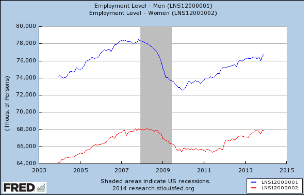
Following the housing bubble-driven recession of 2008 (this is the exposure), the US economy lost a lot of jobs. Here is a graph showing the number of people who were working (the outcome) before, during, and after the recession. Results are being presented stratified by gender (a covariable), meaning the analyst suspected that gender might be acting as an effect modifier. Indeed, the results are slightly different: men (in blue) lost a greater proportion of jobs, and as of 2014 had not yet recovered to pre-recession levels, whereas women (in red) lost fewer jobs and by 2014 had fully recovered.
What if we also stratify by age? First, here is a graph showing how the recession affected jobs for people ages 55 and older:
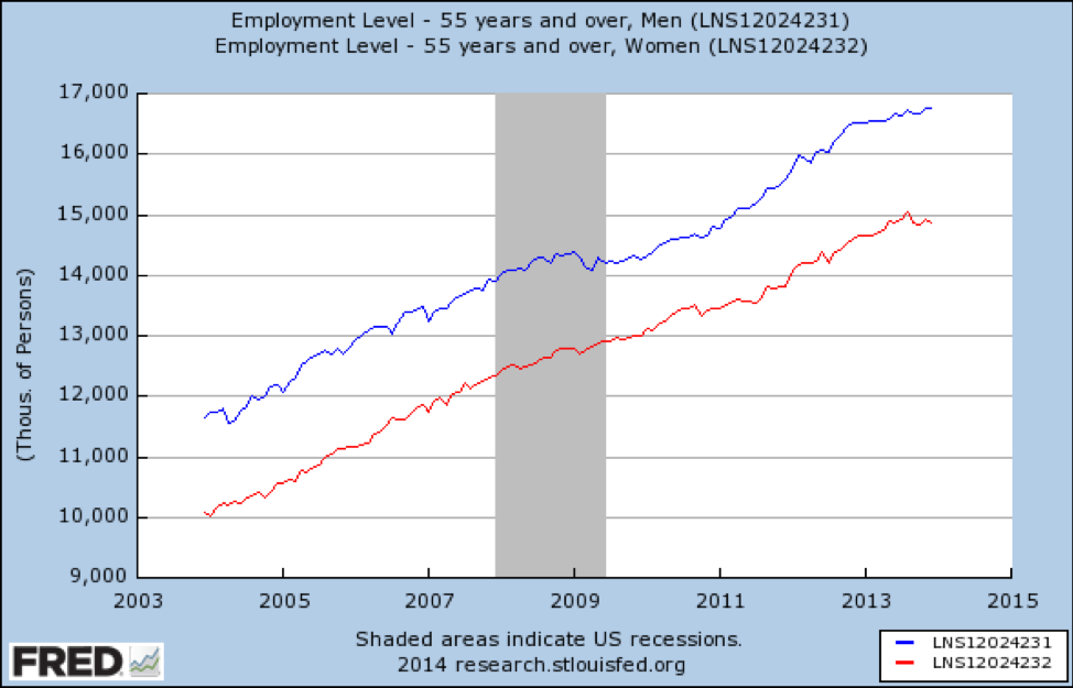
The recession did not affect older working Americans at all. Nor are we seeing effect modification by gender—the 2 lines are nearly parallel.
What about young adults?
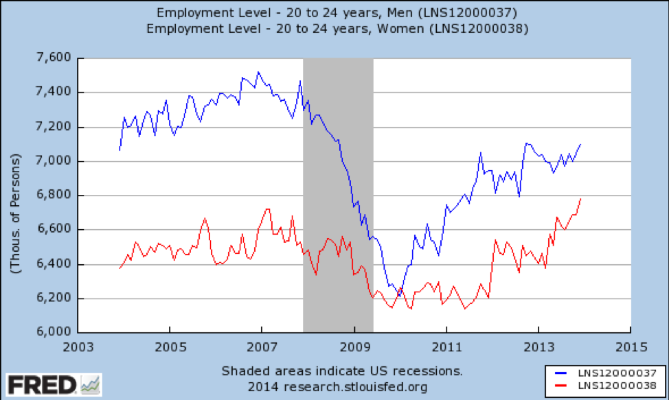
Here we have major effect modification by gender—young men lost a huge proportion of available jobs and had not recovered fully as of 2014. This is not surprising, as the recession was caused largely by the housing bubble, and construction workers are mostly young men. By contrast, young women lost a small proportion of jobs and quickly recovered to better-than-prerecession levels.
Finally, we look at jobs for 25 to 54-year-olds:
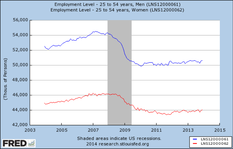
Here we see a very bleak picture. In this age group, jobs were lost—more for men than women—and as of 2014 had not recovered at all.
Thus when examining the job market’s response to the 2008 recession, we see substantial effect modification by age (jobs recovery varied drastically by age) and, within some age categories, also some evidence of effect modification by gender. The effects of the recession on jobs were different for people of different ages and genders.
This is important because the policy implications would be very different. Imagine you were working as part of the federal government and trying to design an economic stimulus or recovery package. If the only data you had came from the first graph, without the age breakdowns, the potential policy solutions would be very different than if you also had access to the stratified-by-age analysis.
Differences between Confounding and Effect Modification
With confounding, you’re initially getting the wrong answer because the confounder is not distributed evenly between your groups. This distorts the measure of association that you calculate (remember: having bigger feet is associated with reading speed only because of confounding by grade level). So instead you need to recalculate the measure of association, this time adjusting for the confounder.
With effect modification, you’re also initially getting the wrong answer, but this time it’s because your sample contains at least 2 subgroups in which the exposure/disease association is different. In this case, you need to permanently separate those subgroups and report results (which may or may not be confounded by still other covariables) separately for each stratum: in this case, men who sleep less have higher GPAs than men who sleep more, but at the same time, women who sleep more have higher GPAs than women who sleep less.
Here is a summary table denoting the process for dealing with potential confounders and effect modifiers. Much of the process is the same regardless of which type of covariable you have (in all cases, you must measure the covariable during your study, and measure it well!). Areas of difference are shown in red.
| Confounding | Effect Modification | |
|---|---|---|
| Before Planning a Study | Think about what variables might act as confounders based on what you know about the exposure/disease process under study. | Think about what variables might act as effect modifiers based on what you know about the exposure/disease process under study. |
| During a Study | Collect data about any potential covariables—stratified/adjusted analyses cannot be conducted without data on the covariable! | Collect data about any potential covariables—stratified/adjusted analyses cannot be conducted without data on the covariable! |
| Analysis: Step 1 | Calculate the crude measure of association (ignoring the covariable). | Calculate the crude measure of association (ignoring the covariable). |
| Analysis: Step 2 | Calculate stratum-specific measures of association, such that each level of the covariable has its own 2 x 2 table. | Calculate stratum-specific measures of association, such that each level of the covariable has its own 2 x 2 table. |
| Analysis: Step 3 | If the stratum-specific measures are similar to each other, and at least 10% different than the crude (which does not fall between them), then the covariable is a confounder. | If the stratum-specific measures are different than each other, and the crude lies between them, then the covariable is an effect modifier. |
| Writing Results | Report an adjusted measure of association that controls for the confounder. | Report the stratum-specific measures of association. |
Example III
Imagine that you do a cross-sectional study of physical activity and dementia in elderly people, and you calculate an unadjusted odds ratio (OR) of 2.0. You think that marital status might be an important covariable, so you stratify by “currently married” versus “not currently married” (which includes never married, divorced, and widowed). The OR among currently married people is 3.1, and among not currently married people the OR is 3.24. In this case, marital status is acting as a confounder, and we would report the adjusted OR (which would be 3.18 or so).
Example IV
Imagine that you do a randomized trial of a Mediterranean diet to prevent preterm birth in pregnant women. You do the trial and calculate an RR of 0.90. You think that perhaps parity might be an important covariable, so you conduct a stratified analysis. Among nulliparas, the RR is 0.60, and among multiparas, the RR is 1.15. These are different than each other, and the crude lies between them. In this case, parity is acting as an effect modifier, and so you would report the 2 stratum-specific RRs separately.
Example V
Imagine that you are doing a case-control study of melanoma and prior tanning bed use. The crude OR is 3.5, but perhaps gender is an important covariable. The stratified analysis yields an OR of 3.45 among men, and 3.56 among women. In this case, the covariable (gender) is neither a confounder nor an effect modifier. We say that it is not a confounder because (1) the crude lies between the 2 stratum-specific estimates, but also (2) the stratum-specific estimates are not more than 10% different than the crude. We say that it is not an effect modifier because, 3.45 and 3.56 are not that different—in both cases, there is a substantial effect (approximately 3.5 times as high). We would report the crude estimate of association, as it requires neither adjustment nor stratification to account for the effects of gender.
Can the Same Variable Act as Both a Confounder and an Effect Modifier?
Yes! Usually we see this when the covariable in question is a continuous variable, dichotomized for the purposes of checking for effect modification. For instance, if we think age might be an effect modifier, we might divide our sample into “old” and “young” for the stratified analysis—say, older than 50 versus 50 or younger. To the extent that 51-year-olds are not like 70-year-olds, we might miss some important nuances in the results, possibly because there exists in the data further effect modification with more categories (which would drop the power to almost nothing, were we to report separately on additional strata) or “residual” confounding as discussed in the previous chapter. Further details are beyond the scope of this book, but know that the same covariable can theoretically act as both a confounder and an effect modifier—but that one rarely sees this in practice.
Conclusion
Unlike confounding, whose effects we want to get rid of in our analysis, effect modification is an interesting finding in and of itself, and we report it. To check for effect modification, conduct a stratified analysis. If the stratum-specific measures of association are different than each other and the crude lies between them, then it’s likely that the variable in question is acting as an effect modifier. Report the results separately for each stratum of the covariable.
One final, put-it-all-together table:
| If these are your ORs/RRs: | ||||
| Crude/Unadjusted | Stratum
1 |
Stratum
2 |
Then the covariable is… | And you would report… |
| 2.0 | 1.0 | 3.2 | an effect modifier | the 2 stratum-specific measures of association |
| 2.0 | 3.5 | 3.6 | a confounder | an adjusted measure |
| 2.0 | 1.9 | 2.0 | nothing interesting | the crude measure |