2.4: Elimination

2.4 Overview of Elimination

Elimination is the combined process of metabolism and excretion. Renal excretion is the primary method by which drugs are removed from the body.

2.4.1 Renal excretion

Along with hepatic metabolism, renal excretion is the other process that eliminates or attenuates the therapeutic action of an absorbed drug. Renal excretion occurs in the kidney as water-soluble compounds are filtered and excreted in the urine. In addition to eliminating water-soluble compounds via passive renal excretion, some compounds are actively transported into the urine by transport proteins that line the tubules of the nephron, which is the functional unit of the kidney. As shown in Figure 2.4.1 below, a simple diagram of a nephron, glomerular filtration takes place in Bowman's capsule, which is the first step of the process. Drugs with a low molecular weight will be freely filtered from the plasma to the glomerulus. An individual's glomerular filtration rate (GFR) determines how much plasma is filtered per unit of time and potentially how quickly a drug is renally eliminated. Another process of renal elimination is tubular reabsorption. Reabsorption of unionized drugs that are weak acids and bases can occur by passive diffusion. Reabsorption may be affected by alterations in urinary pH and ionization. For example, alkalinization of the urine will result in less of the ionized form of an acidic drug being reabsorbed and hence eliminated. Tubular secretion involves two systems to transport organic acids (OAT) and bases (OBT) that may secrete drugs into the ultrafiltrate. The transporters can bind to multiple drugs and other molecules. Thus, they are a site for potential drug-drug interactions because they may compete with each other for binding sites on the transporter.

Figure 2.4.1: Renal Excretion. (CC-BY 4.0; Riley Cutler)

2.4.2. Other pathways of drug elimination

Renal excretion accounts for the vast majority of the elimination of drugs from the body. Other excretion pathways include biliary, respiratory, and mammary excretion, or excretion via sweat or saliva. These non-renal pathways account for a minority of drug elimination from the body and, with only a few exceptions, are relatively insignificant in excretion.

Pharmacokinetic patterns of drug elimination can follow a few different patterns: zero-order, first-order, Michaelis-Menten, and half-life. Each pattern is described visually and in the text.

Zero-order kinetics: A drug following a zero-order pharmacokinetic elimination pattern is eliminated at a constant rate, independent of plasma drug concentration. Drugs that follow zero-order kinetics include aspirin, fluoxetine, thiopental, and omeprazole. Figure 2.4.2.1 demonstrates a zero-order pattern of elimination, which is simply a horizontal line across drug concentrations.

Figure 2.4.2.1: Graph Illustrating Zero-order Kinetics Rate of Elimination Pattern. (CC-BY 4.0; Riley Cutler)

First-order kinetics: When a drug follows a first-order elimination pattern, the rate of elimination depends on the plasma concentration. As the drug plasma concentration increases, so does the rate of elimination. Most medications follow a first-order kinetics pattern of elimination. Figure 2.4.2.2 demonstrates a first-order pattern, which shows that a constant fraction or proportion of the drug is eliminated per unit of time.

Figure 2.4.2.2: Graph Illustrating First-order Kinetics Rate of Elimination Pattern. (CC-BY 4.0; Riley Cutler)

Michaelis-Menten kinetics: In this pattern of pharmacokinetics, the drug’s elimination follows a first-order pattern up to a point, and then it follows a zero-order pattern. The Michaelis-Menten pattern is observed when processes involved in eliminating a drug from the body are saturable. When these processes are saturated, metabolism or excretion can no longer increase to accommodate higher drug concentrations, as demonstrated by the straight line or plateau on the graph. Usually, the number of available transport proteins affects saturation as a transport protein is needed for the drug to move from the circulation into the lumen of the nephron. This pattern is less commonly observed. Note that, as Figure 2.4.2.3 demonstrates, drugs following this type of elimination pattern will take longer to eliminate at higher concentrations. Phenytoin is an example of a medication that follows this pattern.

Figure 2.4.2.3: Graph Illustrating Michaelis-Menten Kinetics Rate of Elimination Pattern. (CC-BY 4.0; Riley Cutler)

Elimination half-life (t1/2): A drug's half-life (t1/2) is a measure of time. Specifically, it is the time it takes for the concentration of a drug to be reduced by half. This parameter helps determine medication dosing intervals and understand how long a drug may remain at physiologically important plasma concentrations. Figure 2.4.2.4 illustrates how a clinician can use the half-life parameter of a drug to estimate how much medication may remain after a dose. After one half-life, 50% of the original concentration remains; after two half-lives, 25% of the original concentration remains; after three half-lives, 12.5% of the original concentration remains. The concentration continues to decrease by half each time the drug’s half-life has elapsed.

Figure 2.4.2.4: Graph Illustrating First-order Kinetics Elimination Half-Life (t1/2). (CC-BY 4.0; Amy Hoang)

2.4.3 Steady State

The steady-state concentration is achieved when the amount of drug coming into the body equals the amount cleared from the body. The plasma concentration is consistent at steady-state concentration, neither rising nor falling. The time it takes for a drug to reach a steady state concentration depends on its elimination pharmacokinetics. One of the simplest ways to conceptualize the time it takes to get to steady-state concentration is to relate this time to the drug’s half-life. The series of figures shown in Figure 2.4.3 panels A-F below depicts a continuous drug infusion starting at time zero through achieving a steady-state concentration. The graphs show the change in plasma concentration over time until a steady state is reached and drug concentration plateaus as the same amount of drug is being administered and leaving the body.

A. The medication concentration is zero before starting an intravenous infusion medication.

B. The plasma concentration rises once the medication infuses (yellow area).

C. The plasma concentration levels off when the drug reaches a “steady state” (green area).

D. Consider points A, B, and C. At point A, the slope of the curve is a steep incline. The plasma concentration is relatively low. The rate of absorption/administration greatly exceeds the rate of elimination.

E. At point B, the slope of the curve is less steep. The plasma concentration is higher, and the elimination rate is closer to the rate of absorption/administration.

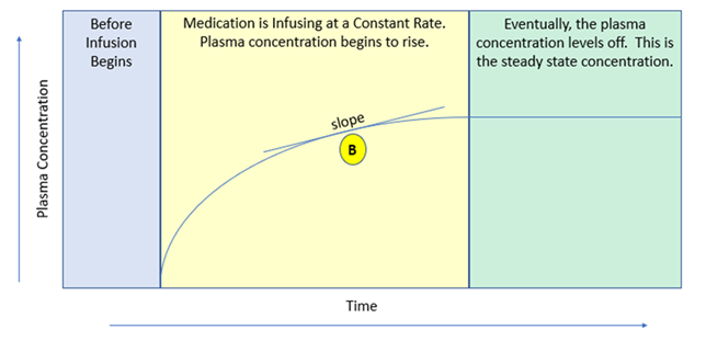
F. At point C, the slope of the curve is flat. At this higher plasma concentration, the elimination rate is equal to the rate of absorption/administration. At this stage, the plasma concentration will stay constant unless there is a change in the administration rate or the body’s ability to clear the drug.

Figure 2.4.3.1 Panels A-F: Graph series illustrating achieving a steady state over time. (CC-BY 4.0; Riley Cutler)

---

This chapter titled 2.4 Elimination is shared under a CC BY-NC-SA 4.0 license and was authored, remixed, and/or curated by Adam Bursa and Karen Vuckovic from Introduction to Pharmacology by Carl Rosow, David Standaert, & Gary Strichartz (MIT OpenCourseWare) via source content that was edited to the style and standards of the LibreTexts platform; a detailed edit history is available upon request. Figures by Riley Cutler and Amy Hoang.