1.2: Epidemiology
- Page ID
- 40925
\( \newcommand{\vecs}[1]{\overset { \scriptstyle \rightharpoonup} {\mathbf{#1}} } \)
\( \newcommand{\vecd}[1]{\overset{-\!-\!\rightharpoonup}{\vphantom{a}\smash {#1}}} \)
\( \newcommand{\dsum}{\displaystyle\sum\limits} \)
\( \newcommand{\dint}{\displaystyle\int\limits} \)
\( \newcommand{\dlim}{\displaystyle\lim\limits} \)
\( \newcommand{\id}{\mathrm{id}}\) \( \newcommand{\Span}{\mathrm{span}}\)
( \newcommand{\kernel}{\mathrm{null}\,}\) \( \newcommand{\range}{\mathrm{range}\,}\)
\( \newcommand{\RealPart}{\mathrm{Re}}\) \( \newcommand{\ImaginaryPart}{\mathrm{Im}}\)
\( \newcommand{\Argument}{\mathrm{Arg}}\) \( \newcommand{\norm}[1]{\| #1 \|}\)
\( \newcommand{\inner}[2]{\langle #1, #2 \rangle}\)
\( \newcommand{\Span}{\mathrm{span}}\)
\( \newcommand{\id}{\mathrm{id}}\)
\( \newcommand{\Span}{\mathrm{span}}\)
\( \newcommand{\kernel}{\mathrm{null}\,}\)
\( \newcommand{\range}{\mathrm{range}\,}\)
\( \newcommand{\RealPart}{\mathrm{Re}}\)
\( \newcommand{\ImaginaryPart}{\mathrm{Im}}\)
\( \newcommand{\Argument}{\mathrm{Arg}}\)
\( \newcommand{\norm}[1]{\| #1 \|}\)
\( \newcommand{\inner}[2]{\langle #1, #2 \rangle}\)
\( \newcommand{\Span}{\mathrm{span}}\) \( \newcommand{\AA}{\unicode[.8,0]{x212B}}\)
\( \newcommand{\vectorA}[1]{\vec{#1}} % arrow\)
\( \newcommand{\vectorAt}[1]{\vec{\text{#1}}} % arrow\)
\( \newcommand{\vectorB}[1]{\overset { \scriptstyle \rightharpoonup} {\mathbf{#1}} } \)
\( \newcommand{\vectorC}[1]{\textbf{#1}} \)
\( \newcommand{\vectorD}[1]{\overrightarrow{#1}} \)
\( \newcommand{\vectorDt}[1]{\overrightarrow{\text{#1}}} \)
\( \newcommand{\vectE}[1]{\overset{-\!-\!\rightharpoonup}{\vphantom{a}\smash{\mathbf {#1}}}} \)
\( \newcommand{\vecs}[1]{\overset { \scriptstyle \rightharpoonup} {\mathbf{#1}} } \)
\(\newcommand{\longvect}{\overrightarrow}\)
\( \newcommand{\vecd}[1]{\overset{-\!-\!\rightharpoonup}{\vphantom{a}\smash {#1}}} \)
\(\newcommand{\avec}{\mathbf a}\) \(\newcommand{\bvec}{\mathbf b}\) \(\newcommand{\cvec}{\mathbf c}\) \(\newcommand{\dvec}{\mathbf d}\) \(\newcommand{\dtil}{\widetilde{\mathbf d}}\) \(\newcommand{\evec}{\mathbf e}\) \(\newcommand{\fvec}{\mathbf f}\) \(\newcommand{\nvec}{\mathbf n}\) \(\newcommand{\pvec}{\mathbf p}\) \(\newcommand{\qvec}{\mathbf q}\) \(\newcommand{\svec}{\mathbf s}\) \(\newcommand{\tvec}{\mathbf t}\) \(\newcommand{\uvec}{\mathbf u}\) \(\newcommand{\vvec}{\mathbf v}\) \(\newcommand{\wvec}{\mathbf w}\) \(\newcommand{\xvec}{\mathbf x}\) \(\newcommand{\yvec}{\mathbf y}\) \(\newcommand{\zvec}{\mathbf z}\) \(\newcommand{\rvec}{\mathbf r}\) \(\newcommand{\mvec}{\mathbf m}\) \(\newcommand{\zerovec}{\mathbf 0}\) \(\newcommand{\onevec}{\mathbf 1}\) \(\newcommand{\real}{\mathbb R}\) \(\newcommand{\twovec}[2]{\left[\begin{array}{r}#1 \\ #2 \end{array}\right]}\) \(\newcommand{\ctwovec}[2]{\left[\begin{array}{c}#1 \\ #2 \end{array}\right]}\) \(\newcommand{\threevec}[3]{\left[\begin{array}{r}#1 \\ #2 \\ #3 \end{array}\right]}\) \(\newcommand{\cthreevec}[3]{\left[\begin{array}{c}#1 \\ #2 \\ #3 \end{array}\right]}\) \(\newcommand{\fourvec}[4]{\left[\begin{array}{r}#1 \\ #2 \\ #3 \\ #4 \end{array}\right]}\) \(\newcommand{\cfourvec}[4]{\left[\begin{array}{c}#1 \\ #2 \\ #3 \\ #4 \end{array}\right]}\) \(\newcommand{\fivevec}[5]{\left[\begin{array}{r}#1 \\ #2 \\ #3 \\ #4 \\ #5 \\ \end{array}\right]}\) \(\newcommand{\cfivevec}[5]{\left[\begin{array}{c}#1 \\ #2 \\ #3 \\ #4 \\ #5 \\ \end{array}\right]}\) \(\newcommand{\mattwo}[4]{\left[\begin{array}{rr}#1 \amp #2 \\ #3 \amp #4 \\ \end{array}\right]}\) \(\newcommand{\laspan}[1]{\text{Span}\{#1\}}\) \(\newcommand{\bcal}{\cal B}\) \(\newcommand{\ccal}{\cal C}\) \(\newcommand{\scal}{\cal S}\) \(\newcommand{\wcal}{\cal W}\) \(\newcommand{\ecal}{\cal E}\) \(\newcommand{\coords}[2]{\left\{#1\right\}_{#2}}\) \(\newcommand{\gray}[1]{\color{gray}{#1}}\) \(\newcommand{\lgray}[1]{\color{lightgray}{#1}}\) \(\newcommand{\rank}{\operatorname{rank}}\) \(\newcommand{\row}{\text{Row}}\) \(\newcommand{\col}{\text{Col}}\) \(\renewcommand{\row}{\text{Row}}\) \(\newcommand{\nul}{\text{Nul}}\) \(\newcommand{\var}{\text{Var}}\) \(\newcommand{\corr}{\text{corr}}\) \(\newcommand{\len}[1]{\left|#1\right|}\) \(\newcommand{\bbar}{\overline{\bvec}}\) \(\newcommand{\bhat}{\widehat{\bvec}}\) \(\newcommand{\bperp}{\bvec^\perp}\) \(\newcommand{\xhat}{\widehat{\xvec}}\) \(\newcommand{\vhat}{\widehat{\vvec}}\) \(\newcommand{\uhat}{\widehat{\uvec}}\) \(\newcommand{\what}{\widehat{\wvec}}\) \(\newcommand{\Sighat}{\widehat{\Sigma}}\) \(\newcommand{\lt}{<}\) \(\newcommand{\gt}{>}\) \(\newcommand{\amp}{&}\) \(\definecolor{fillinmathshade}{gray}{0.9}\)Epidemiology is defined as the study of human populations. These studies often investigate the relationship between dietary consumption and disease development. There are three main types of epidemiological studies: cross-sectional, case-control, and prospective cohort studies.
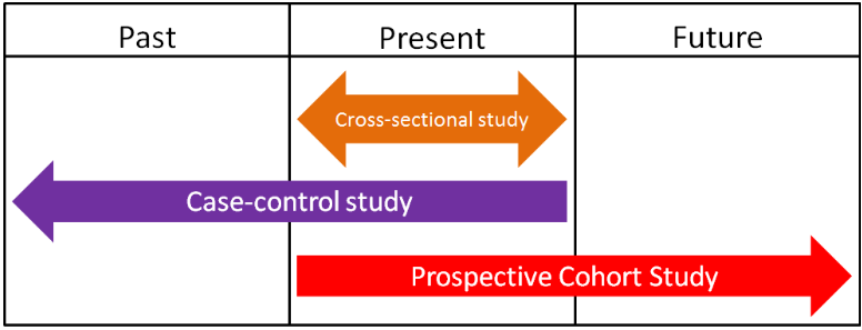
Cross-Sectional Studies
Cross-sectional studies compare different populations at the same point in time. It is as if you take a snapshot of the two different populations to compare them to one another. An example of a cross-sectional study led to a phenomenon known as the "French Paradox." Cholesterol and saturated fat intake were associated with increased risk of coronary heart disease across a wide variety of countries. However, within the study they noticed a surprising result. European countries with very similar cholesterol-saturated fat intakes had hugely different death rates from coronary heart disease deaths, as shown below.

The French had a 5-fold lower risk of dying from coronary heart disease than the Finns, despite having similar cholesterol-saturated fat intakes2. A paradox means something contradictory, which this finding seemed to be. The "French Paradox" has led to research on red wine, and one of its active components, resveratrol, because the French consume a lot of this alcoholic beverage. Cross-sectional studies are considered the weakest type of epidemiology because they are based only on group outcomes. This may lead people to believe that members of the group have characteristics, which as individuals they do not. This is known as ecologic (another name that is used to refer to this type of study) fallacy, and is a limitation of cross-sectional studies3.
Query \(\PageIndex{1}\)
Case-Control Studies
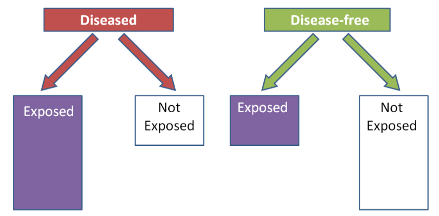
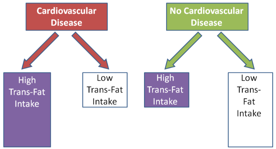
Case-control studies look at a group of cases (e.g. people with a disease) vs. controls (e.g. people without the disease). Most case-control studies are retrospective (looking back in time, or looking at the past). These studies try to determine if there were differences in the diets of the cases compared to controls in the past. Cases and controls are matched on characteristics such as age, sex, BMI, history of disease, and many others. This means researchers try to choose a control that has similar characteristics to the case. The researchers then compare the exposure levels between cases and controls, as shown below. In this example a greater proportion of diseased (cases) individuals than disease-free individuals (controls) were exposed to something.
Using trans-fat intake as the exposure, and cardiovascular disease as the disease, the figure would be expected to look like this:
To determine people's intakes of foods and food components, food frequency questionnaires are commonly used. As the name suggests, a food frequency questionnaire is a series of questions that determines how frequently you consume a certain food. An example of a question on a food frequency questionnaire is shown below:
"Over the past 12 months, how often did you drink milk?"
- Never
- 1 time/month less
- 2-3 times/month
- 1-2 times/week
- 3-4 times/week
- 5-6 times/week
- 1 time/day
- 2-3 times/day
- 4-5 times/day
- 6 or more times/day
An example of a food frequency questionnaire is shown in the link below.
Web Link
Query \(\PageIndex{2}\)
Prospective Cohort Studies
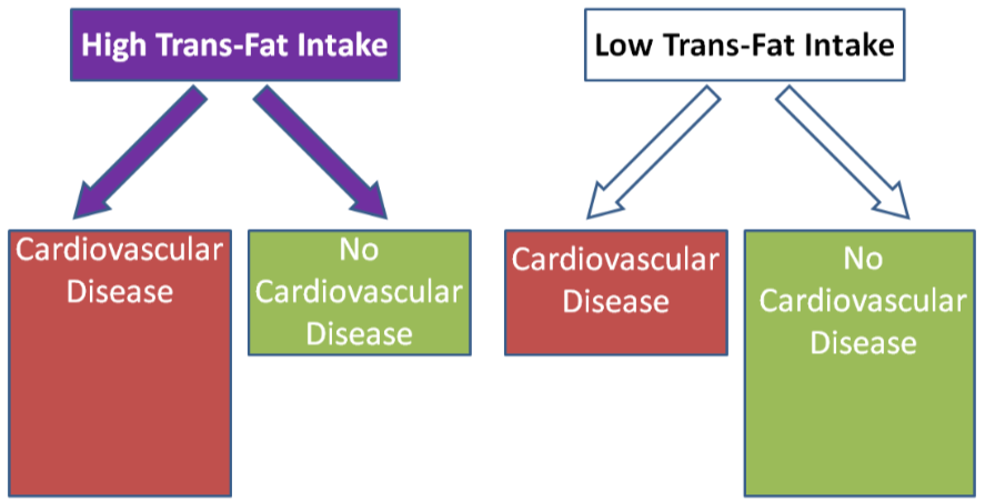
A cohort is "a group of subjects." Most cohort studies are prospective. Initial information is collected (usually by food frequency questionnaires) on the intake of a cohort of people at baseline, or the beginning. This cohort is then followed over time (normally many years) to quantify health outcomes of the individual within it. Cohort studies are normally considered to be more robust than case-control studies, because these studies do not start with diseased people and normally do not require people to remember their dietary habits in the distant past or before they developed a disease. An example of a prospective cohort study would be if you filled out a questionnaire on your current dietary habits and are then followed into the future to see if you develop osteoporosis. As shown below, instead of separating based on disease versus disease-free, individuals are separated based on exposure. In this example, those who are exposed are more likely to be diseased than those who were not exposed.
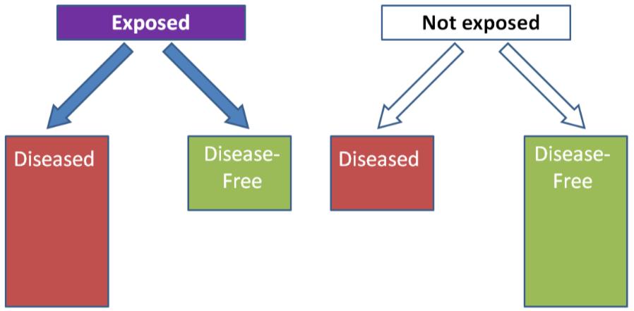
Using trans-fat intake again as the exposure and cardiovascular disease as the disease, the figure would be expected to look like this:
There are several well known examples of prospective cohort' studies as listed below.
Framingham Heart Study
The Framingham Heart Study started in 1948 and has been following the residents of Framingham, Massachusetts to identify risk factors for heart disease. This cohort has been very fruitful in finding a number of important factors associated with coronary heart disease. In 2002, a third generation of participants was enrolled to be followed. The following links show more about the Framingham Heart Study
Nurses Health Study
The Nurses’ Health Study started in 1976 and enrolled 122,000 female nurses. Every 4 years they received a food frequency questionnaire to assess their dietary habits.
Web Link
Health Professionals Follow-Up Study
The Health Professionals Follow-Up Study started in 1986 and enrolled 51,529 male health professionals (dentists, pharmacists, optometrists, osteopathic physicians, podiatrists, and veterinarians). Every 4 years they received a food frequency questionnaire to assess their dietary habits.
Web Link
The Health Professionals Follow-Up Study is a good example for how cohort studies can be important in nutrition research. We will consider one example in which the researchers administered food frequency questionnaires that contained 131 food and beverage items to determine whether their intake was associated with increased or decreased risk of developing prostate cancer. Of these items, intake of four foods (tomatoes, tomato sauce, pizza, and strawberries) were associated with decreased incidence of prostate cancer, as illustrated in the figure below4.

The three tomato-based foods are red due to the presence of the carotenoid lycopene. Strawberries don't contain lycopene (their red color is due to anthocyanins). This finding has led to interest in the potential of tomatoes/lycopene to decrease the risk of prostate cancer.
Query \(\PageIndex{3}\)
Query \(\PageIndex{4}\)
Query \(\PageIndex{5}\)
References
- Levin K. (2006) Study design III: Cross-sectional studies. Evidence - Based Dentistry 7(1): 24.
- Artaud-Wild SM, Connor SL, Sexton G, Connor WE. (1993) Differences in coronary mortality can be explained by differences in cholesterol and saturated fat intakes in 40 countries but not in france and finland. A paradox. Circulation 88(6): 2771.
- Gordis L. (2004) Epidemiology. Philadelphia, PA: Elsevier Saunders.
- Giovannucci E, Ascherio A, Rimm EB, Stampfer MJ, Colditz GA, et al. (1995) Intake of carotenoids and retinol in relation to risk of prostate cancer. J Natl Cancer Inst 87(23):1767-1776.


